On an interval prediction of COVID-19 development based on a SEIR epidemic model

Abstract

In this paper, a new version of the well-known epidemic mathematical SEIR model is used to analyze the pandemic course of COVID-19 in eight different countries. One of the proposed model’s improvements is to reflect the societal feedback on the disease and confinement features. The SEIR model parameters are allowed to be time-varying, and the ranges of their values are identified by using publicly available data for France, Italy, Spain, Germany, Brazil, Russia, New York State (US), and China. The identified model is then applied to predict the SARS-CoV-2 virus propagation under various conditions of confinement. For this purpose, an interval predictor is designed, allowing variations and uncertainties in the model parameters to be taken into account. The code and the utilized data are available on Github.

1. Introduction

The SEIR model is one of the simplest compartmental models of epidemics (Keeling & Rohani, 2008). It is a very popular model and is extensively used in various settings (Wang et al., 2016). The SEIR model represents the development of the relative proportions of four classes of individuals in a population of constant size: the susceptible individuals $S$, capable of contracting the disease and becoming infectious; the asymptomatic (or exposed) $E$ and symptomatic $I$ infectious, capable of giving the disease to susceptible; and the recovered $R$, permanently immune after healing or dying (if the number of deaths is of particular interest, then an additional compartment $D$ can be included). This simple model depicts a generic behavior of epidemics (as a series of transitions between these compartments), and a related advantage consists of a small number of parameters to be identified (three transition rates $\sigma$, $\gamma$, and $b$). This latter is an essential point in a virus attack when an insufficient amount of data is available. In May 2020, when the present paper was written, that was mainly the situation worldwide under the SARS-CoV-2 virus’s presence.

There exist many sorts and varieties of SEIR models (Keeling & Rohani, 2008) (e.g., in the most simplistic case, the classes $E$ and $I$ are modeled at once, leading to a SIR model). A specificity of COVID-19 pandemics is the global confinement imposed by most countries worldwide, influencing the virus dynamics (Das, Ghosh, Sen, & Mukhopadhyay, 2020). In recent literature, numerous approaches propose how to reflect the confinement characteristics in the mathematical models (Dandekar and Barbastathis, 2020, Lopez and Rodo, 2020, Nussbaumer-Streit et al., 2020). In Efimov and Ushirobira (2020), we propose a slightly similar SEIR model to analyze the course of SARS-CoV-2 in France.

This work aims to use a novel SEIR model to predict the outbreak development with different quarantine restrictions. Our preliminary attempts to identify such model parameters confirmed that their constancy hypothesis is very restrictive, motivating us to consider time-varying parameters (not much analyzed in the literature). An interval predictor is then designed to realize an efficient and reliable prediction for a SEIR model with time-varying parameters, whose set-membership forecasting abilities perfectly suit the considered scenario. The stability of the predictor and its inclusion capabilities are analytically evaluated. The performance of the proposed approach is shown in numerical experiments for some countries.

The plan of this paper is as follows. The new modified SEIR epidemic model is presented in Section 2, together with an analysis of the model parameters and their admissible values ranges, found in the literature. In Section 3, we describe the measured data applied for the parameter identification and some hypotheses used in the sequel (we fix the values of some parameters having a “physical” meaning in order to be able to identify the remaining ones). The method for parameter identification is presented in Section 4. An interval predictor is designed in Section 5, allowing us to evaluate the present situation under the variation of parameters and initial states. The application results of the proposed identification routine and the interval predictor are given in Section 6 for France, Italy, Spain, Germany, Brazil, Russia, New York State (US), and China. The accuracy of the interval prediction is also evaluated using data for identification and another part for verification. Final discussions and remarks are provided in Section 7.

2. Epidemic model and considerations

This paper proposes a modified SEIR discrete-time model based on the one in Yang et al. (2020), where it has been used to model the course of the epidemic of COVID-19 in China (other similar SIR/SEIR-type models used recently for modeling SARS-CoV-2 virus can be found in Ferguson et al., 2020, Gevertz et al., 2020, Lourenco et al., 2020, Maier and Brockmann, 2020, Peng et al., 2020). The model we propose in this work is as follows (the impact of the natural birth and mortality is not considered, since, for the short period of analysis studied here, the population may be assumed quasi-constant):

$$S_{t+1}=S_t-b\frac{\left(p_{t-{\tau }_p}{I}_t+r_{t-{\tau }_r}{E}_t\right)}{N}{S}_t,$$ (1a)

$$E_{t+1}=(1-\sigma -{\sigma }^{\prime })E_t+b\frac{\left(p_{t-{\tau }_p}{I}_t+r_{t-{\tau }_r}{E}_t\right)}{N}{S}_t,$$ (1b)

$$I_{t+1}=(1-\gamma -\mu )I_t+\sigma E_t,$$ (1c)

$$R_{t+1}=R_t+\gamma I_t+{\sigma }^{\prime }{E}_t,$$ (1d)

$$D_{t+1}=D_t+\mu I_t,$$ (1e)

where $t\in \mathbb{N}$ (the set of non-negative integers) is the time counted in days ($t=0$ corresponds to the beginning of measurements or prediction), $N=S+E+I+R+D$ denotes the total population, the parameter $0<\gamma <+\infty$ represents the recovery rate, $0<\mu <+\infty$ is the mortality rate, the parameter $0<b<+\infty$ corresponds to the rate of the virus transmission from infectious/exposed to susceptible individuals during a contact, $0<\sigma ,{\sigma }^{\prime }<+\infty$ are the incubation rates at which the exposed develop symptoms or directly become recovered without a viral indication, $0\le p_t<+\infty$ corresponds to the number of contacts for the infectious $I$ (it is supposed that infected people with symptoms are in quarantine, then the number of contacts is decreased), $p_t\le r_t<+\infty$ is the number of contacts per person per day for the exposed population $E$ (in the presence of confinement and depending on its severity, this number is time-varying), and ${\tau }_p,{\tau }_r>0$ are the delays in the reactions of the compartments on variations of quarantine conditions (we assume that if $t<{\tau }_p$ or $t<{\tau }_r$, then $p_{t-{\tau }_p}=p_0$ or $r_{t-{\tau }_r}=r_0$, respectively). Compared to the model in Yang et al. (2020), the inflow/outflow variables from/to other regions for each state are not considered in our analysis.

In the model (1), for the brevity of introduction, we assume that the parameters $\sigma$, ${\sigma }^{\prime }$, $\gamma$, $\mu$ and $b$ have constant values, and we revisit this hypothesis later.

2.1. Societal feedback and confinement influence in the model

To consider society’s reaction to confinement and virus propagation, we introduce the delays ${\tau }_p$ and ${\tau }_r$ in the seclusion inputs $p_t$ and $r_t$, respectively.

The idea behind ${\tau }_r$ is that after the quarantine activation, several days pass before changes in the disease propagation become detectable (such an effect can be easily observed in the data for all analyzed countries). Roughly speaking, the increase in the number of infected individuals $E$ and $I$ is predefined by the number of contacts in the previous days, when the confinement was not yet imposed, for example.

We assume that during the phase of active lockdown, $r_{t-{\tau }_r}=p_{t-{\tau }_p}$ always holds, i.e., the number of contacts for asymptomatic $E$ and symptomatic $I$ infected populations is the same (when the society follows Governments requirements).

The delay ${\tau }_p$ is used to model the clustering effect of the confinement: under restrictions on displacement activities, people are compelled to stay in their neighborhood and visit a limited number of attractions (such as shops, pharmacies, hospitals). So the population can be considered to be divided into smaller groups. After some time the chances to meet an infected person start to decay (e.g., there is no infected person in such a group, or the individual was isolated, or the whole group can be infected, but in any case, the virus propagation is almost stopped).

Remark 1

A different way of including societal feedback on the current SARS-CoV-2 virus development is the substitution:

$$b⟶\frac{b}{1+\eta I_t},$$

where $0<\eta <+\infty$ is a tuning parameter. In this case, we model the effect of natural augmentation of confinement strictness. Many factors can lead to this increase; for instance, society becomes aware of the problem following the increased number of infected or dead people (the variable $I$ implicitly represents them, or it can also be explicitly replaced with $D$). To this end, we decrease the virus transmission rate $b$ with the growth of the number of infected/dead individuals. This variant has been tested, but we prefer to use the delays ${\tau }_p$ and ${\tau }_r$ since, in this case, the parameter identification is more straightforward.

Compared to our proposed model, the main shortcoming of other models in the literature is that they do not consider the societal feedback and delays in their computation. The countries examined in the present paper have adopted different policies all through the pandemics, and to consider such factor seems indeed quite valuable.

2.2. Model parameters

Therefore, the SEIR model (1) has seven parameters to be identified or assigned: $\sigma$, ${\sigma }^{\prime }$, ${\tau }_p$, ${\tau }_r$, $\gamma$, $\mu$ and $b$.

2.2.1. Generic observations

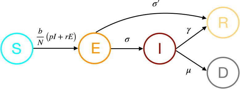
The parameters $\sigma$, ${\sigma }^{\prime }$, $\gamma$, $\mu$ and $b$ represent, respectively, the rate of changes between the states $E$ to $I$, $E$ to $R$, $I$ to $R$, $I$ to $D$ and $S$ to $E$ (as in Fig. 1). The parameters $\sigma$ and ${\sigma }^{\prime }$ have a physical meaning: $\sigma =\frac{1}{T_S}$ and ${\sigma }^{\prime }=\frac{\kappa }{T_S}$, where $T_s$ is the average duration of the virus incubation period after contamination, which can be well identified in patients, and $\kappa \in [0,1)$ is the ratio of recovering period for the patients with the mild form of COVID-19, which can also be found in sufferers. Similarly, the delays ${\tau }_r$ and ${\tau }_p$ are of order $T_s$, and have a natural origin. The numbers of contacts in $p_t$ and $r_t$ (with or without (relaxed) confinement) can be evaluated heuristically based on the population density and social practices (for prediction, different profiles can be selected for testing).

Fig. 1.

A schematic representation of our new modified SEIR model.

2.2.2. Known or accepted quantities

The incubation period $T_s$ that is widely papered in the literature for COVID-19 studies, is considered to be between $2$ and $14$ days (Yang et al., 2020), or in more specialized research, between $2$ and $12$ days (Lauer et al., 2020), so we assume

$$\frac{1}{12}\le \sigma \le \frac{1}{2}.$$

It also implies that the delays can be selected in the corresponding limits:

$$2\le {\tau }_r\le 12,{\tau }_r+2\le {\tau }_p,$$

where the condition ${\tau }_p>{\tau }_r$ entails that the clustering starts to be important after the effect of confinement becomes significant (adding an incubation period).

The numbers of contacts have to be selected separately for each country. For example, we may take the values of Yang et al. (2020) and make some reduction related with a smaller population density in the considered countries:

$$p_Q=3\text{ (number of contacts in quarantine)},$$

$$p_N=15\text{ (number of contacts in normal mode)},$$

$$p_R=10\text{ (number of contacts in relaxed quarantine)},$$

$$p_C=0.1\text{ (number of contacts under clustering).}$$

Then the input $p_t\in \{p_Q,p_C\}$ and $r_t\in \{p_Q,p_N,p_R,p_C\}$ for all $t\in \mathbb{N}$.

The identification of the model parameters may be performed using statistics published by authorities.1 As a worthy remark, many research works devoted to the estimation and identification of SIR/SEIR models were developed by now, and several in the last few years, such as Bliman et al., 2018, Cantó et al., 2017, d’Onofrio et al., 2012, Magal and Webb, 2018 and Ushirobira, Efimov, and Bliman (2019), to mention a few.

2.3. Uncertainty and prediction

Since the measured data and parameters contain numerous uncertainties and perturbations, it is challenging to carry out a reasonable prediction based on the simulation of such a model with fixed parameters (also considering the model simplicity and generality). However, the interval predictor and observer framework (Efimov and Raïssi, 2016, Gouzé et al., 2000, Mazenc and Bernard, 2011, Mazenc et al., 2014, Raïssi et al., 2012) allows a set of trajectories corresponding to the interval values of parameters and inputs to be obtained, increasing the model validity without augmenting its complexity. This approach has already been applied to different SEIR models (see, e.g., Aronna and Bliman, 2018, Degue et al., 2016, Degue and Le Ny, 2018). In this paper, we apply the interval predictor method for the considered SEIR model (1) to improve its forecasting quality by assuming that the parameters $\sigma$, ${\sigma }^{\prime }$, $\gamma$, $\mu$ and $b$ are time-varying.

Remark 2

It is essential to emphasize that the interval predictor framework used here is not the only method oriented toward improving prediction reliability when using SEIR models. Usually, as in Ferguson et al., 2020, Hu et al., 2020, Lourenco et al., 2020, Maier and Brockmann, 2020, Peng et al., 2020 and Yang et al. (2020), stochastic and agent-based simulation procedures are used. In those cases, by assuming that the parameters and initial conditions are distributed with some given probability, multiple numerical experiments are done to restore the system’s possible trajectories. Such a methodology needs more computational effort for its realization. Additional information on the probability distribution for all parameters and variables is necessary, demanding either extra hypotheses or more measured data for estimation. As the SARS-CoV-2 virus attack currently demonstrates, it is difficult to obtain such data quickly during the epidemic development. Contrarily to these approaches, the interval predictor method does not use these extra assumptions on probability distributions. It has also been proposed to estimate a guaranteed interval, including trajectories with minimal computational effort, by the cost of a more complex mathematical analysis and design (Efimov & Raïssi, 2016).

3. Used dataset and associated parameters

Let $ℐ$, $\mathcal{D}$, and $ℛ$ represent the number of total detected infected, deceased and recovered individuals, respectively (these information are published by authorities). Not all cases can be detected and documented by public health services, so there is a ratio between populations $I$ and $ℐ$, $R$ and $ℛ$, $D$ and $\mathcal{D}$, which is denoted in this work by $\alpha$. The interval of admissible values for $\alpha$ is estimated from different sources as follows2 :

$$1\le \alpha \le 25.$$

Formally, such a ratio $\alpha$ has to be time-varying and different for $I$, $D$ and $R$. Due to strict and similar requirements of health services in almost all considered countries, in this paper, we take the following hypotheses:

$$I_t={\alpha }_1({ℐ}_t-{\mathcal{D}}_t-{ℛ}_t),R_t={\alpha }_2{ℛ}_t,D_t={\alpha }_3{\mathcal{D}}_t,$$ (2)

i.e., the number of active infected cases and the related recovered individuals can be masked due to the complexity of examination and the actual confirmation of the virus presence. At the same time, the availability or not of post-mortem tests can influence the number of registered deaths. A further reason is that in many cases, the virus symptoms result in a mild reaction of patients (approximately 80% of cases, see the sources above), hence maybe with no official virus confirmation in such a situation. In this work, we assume the following values for these parameters:

$${\alpha }_2={\alpha }_1,{\alpha }_3=1,$$

then, roughly speaking, such a choice corresponds to the registration of deaths exactly (see also Lourenco et al., 2020) with the same error for recovered and infected individuals (the exclusion was made only for the US). CMMID describes a technique to identify ${\alpha }_1$ from the measurements of $ℐ$, $ℛ$ and $\mathcal{D}$ (see the footnote) giving for France (in July 30th):

$${\alpha }_1=1.78.$$

So, by fixing ${\alpha }_1$, ${\alpha }_2$, and ${\alpha }_3$,3 the three variables of the model (1), $I$, $D$, and $R$, are available from the beginning of the epidemics via (2).

Remark 3

The measured information used in the paper are $I$, $R$, and $D$ from (2), where the measurement noise can be modeled by time-varying gains ${\alpha }_i$, $i=1$, $2$, $3$, representing the different actual values of populations in these compartments. Such noise characteristics are in general unknown (country dependent), and it is difficult to estimate them during the outbreak. However, if we assume that the noise is bounded, then instead of the exact values of $I$, $R$, and $D$, their intervals have to be considered, $[\underset{\_}{I},\overline{I}]$, $[\underset{\_}{R},\overline{R}]$, and $[\underset{\_}{D},\overline{D}]$, corresponding to possible true values of these variables. Using such intervals would lead to interval estimates for parameters (with the methods applying below). To simplify the presentation and the computations, it is assumed in this work that the measured quantities in (2) are noise-free, resulting in the identification of guess values for the parameters. Finally, for prediction, the intervals around the guesses are calculated for all initial conditions, parameters and inputs, which takes into account the presence of the noise in (2) and other uncertainties or complexity effects.

3.1. Fixed values of parameters

Note that model (1) is not identifiable with respect to all seven parameters simultaneously for the given set of measured outputs ($I$, $R$, and $D$) and inputs ($p$ and $r$). Hence, it is necessary to fix the values of some of them, those with a physical meaning, for instance, and reconstruct the sets of admissible values for others. To this end, we select an average value for the incubation rate:

$$\sigma =\frac{1}{7}$$

to simplify further identification (the variation in this value can be taken into account later in the interval predictor), then

$${\sigma }^{\prime }=\kappa \sigma ,\kappa =0.1,$$

and we assume that there is a very slow transfer from exposed $E$ to recovered $R$ directly without symptom exposition. The delays’ nominal values are chosen as

$${\tau }_r=5,{\tau }_p={\tau }_r+20,$$

and the algorithm for their identification is discussed below. The procedure for identifying $\gamma$, $\mu$, and $b$ is also given in the next section.

3.2. Scenario of confinement

In Ferguson et al. (2020), the theory of a cyclic application of quarantine regimes of different severity is evaluated for COVID-19. By iterating the periods of complete isolation for everybody (suppression), which decelerates the virus advancement, with a time of mild regulation (mitigation), which allows the economy balance to be maintained on an arguable level, and when only fragile parts of the population are isolated, it is possible to attenuate the material consequences of epidemics while decreasing the load on health services. Following this idea, for simulation, we consider a cyclic scenario of confinement (e.g., with $8$ weeks of strict quarantine and $4$ weeks of a relaxed one), which is further periodically repeated. For the chosen model, this scenario impact only the input variables $p_{t-{\tau }_p}$ and $r_{t-{\tau }_r}$, an example of their behavior is shown in Fig. 2 (by red dash and blue solid lines, respectively).

Fig. 2.

Variation of the number of contacts $p_{t-{\tau }_p}$ and $r_{t-{\tau }_r}$.

Remark 4

In other words, $r_t$ and $p_t$ can be considered as a sort of control for the virus propagation, by imposing different periods and strictness levels for the confinement for compartments $I$ and $E$. A more detailed analysis may also take into account age or geographic distribution.

4. Parameter identification

In this section, we assume that the parameters have constant values, which allows us to apply efficient methodologies for their identification. Next, we use these values as the nominal or average quantities passing to time-varying parameters.

For the parameter identification, we assume that the incubation rates $\sigma$ and ${\sigma }^{\prime }$ are fixed as above and that the symptomatic infectious $I_t$, the dead $D_t$, and the recovered $R_t$ persons are measured for the first $J>0$ days of the virus attack as in (2) for $t=0,1,\dots ,J$.

We begin by discussing approaches to the identification of the delays ${\tau }_p$ and ${\tau }_r$. Then, the method for identifying the mortality rate $\mu$, the recovery rate $\gamma$, and the infection rate $b$ is presented. Finally, the model (1) with the parameters’ obtained values is validated by simulations in Section 6.

4.1. Delay identification

We propose two approaches for the estimation of ${\tau }_p$ and ${\tau }_r$.

4.1.1. Method 1

From the dynamics of (1b), the increment of $E_t$ (i.e., $E_{t+1}-E_t$) is directly proportional to $p_{t-{\tau }_p}$ and $r_{t-{\tau }_r}$. The number of contacts $r_{t-{\tau }_r}$ instantaneously changes its value after the imposition of the quarantine (it jumps from $p_N$ to $p_Q$). Since ${\tau }_p>{\tau }_r$ and $p_{t-{\tau }_p}=r_{t-{\tau }_r}$ in confinement, the signals $p_{t-{\tau }_p}$ and $r_{t-{\tau }_r}$ jump next from $p_Q$ to $p_C$, and the same occurs after the suppression of the confinement (from $p_C$ to $p_Q$ or $p_R$), see Fig. 2. It implies that the increment of $E_t$ shows discontinuities in these time instants. The variable $E_t$ is not available for measurements, but the same (filtered) behavior is also observed in the increment of the variable $I_t$. Since both variables, $I_t$ and $E_t$ in (1) have an exponential rate of changes, then the signal

$$d{I}_t=ln\left(I_t\right)-ln\left(I_{t-1}\right)$$

for $t=2,\dots ,J$ should have a step-like form (the logarithm of the increment of an exponentially growing or decaying signal is a constant) with the change of value in the time instant $t_c\ge 2$, when a modification of the confinement rules starts to influence the variable $I_t$. Therefore, the delay can be estimated as (with a mild ambiguity in this work, we use the same symbol to denote a parameter and its estimate)

$${\tau }_r=t_c-t^{\prime },$$

where $t^{\prime }\ge 0$ is the instant of application of the new confinement rule. Hence, to estimate the value $t_c$, the following algorithm is proposed:

$$t_c=\underset{t=3,\dots ,J}{\text{arg}min}\sqrt{\sum _{\ell =2}^J{|d{I}_{\ell }-d{I}_{\ell }^t|}^2},\text{ where }d{I}_{\ell }^t=\left\{\begin{array}{cc}\frac{1}{t-2}\sum _{s=2}^{t-1}d{I}_s\hfill & ,\text{if }\ell <t\hfill \\ \frac{1}{J-t+1}\sum _{s=t}^{J}d{I}_s\hfill & ,\text{if }\ell \ge t\hfill \end{array}\right)$$

is a step-like varying signal, which jumps at the instant $t$. This approach’s main drawback is the noise in the measurements (as for any approach that indirectly uses a derivative estimation).

Remark 5

Note that if the values of $\gamma$ and $\mu$ are known (see below how we can estimate them), then using (1c) the variable $E_t=\frac{1}{\sigma }\left(I_{t+1}-(1-\gamma -\mu )I_t\right)$ can be reconstructed from the measurements, and the same approach can be applied to the increment $d{E}_t=ln\left(E_t\right)-ln\left(E_{t-1}\right)$, which explicitly depends on $p_{t-{\tau }_p}$ and $r_{t-{\tau }_r}$. Unfortunately, we have very noisy data for COVID-19, so the calculated variables $E_t$ contain many perturbations, and the above (derivative-based) approach does not provide a reliable estimation using $d{E}_t$.

4.1.2. Method 2

This method also uses the estimated values of $E_t$ (see (3) for the detailed description), but it does not use (approximated) derivatives. The idea of this approach is based on the observation that a straight line can approximate $ln\left(E_t\right)$ (the variable $E_t$ is exponentially growing) for any constant values of $p_{t-{\tau }_p}$ and $r_{t-{\tau }_r}$:

$$ln\left(E_t\right)=at+b,$$

for some $a,b\in \mathbb{R}$. Such an approximation filters the noise contrarily to the derivative-based method presented in the previous subsection. Then the initial phase of the epidemics can be decomposed on three intervals of time:

$${\mathcal{T}}_1=[0,T_1+{\tau }_r),{\mathcal{T}}_2=[T_1+{\tau }_r,T_1+{\tau }_p),{\mathcal{T}}_3=[T_1+{\tau }_p,T_2],$$

where $T_1$ is the day of confinement activation, $T_2$ is the day of commutation to the relaxed quarantine, and on each interval

$$ln\left(E_t\right)=a_{i}t+b_i,$$

for $t\in {\mathcal{T}}_i$ and some coefficients $a_i,b_i\in \mathbb{R}$ with $i=1,2,3$, is a reliable approximation. The coefficients $a_i,b_i$ can be calculated using the Least Square Method (LSM), or any other approach of solving this system of linear equations with known reconstructed values of $E_t$. Next, we can calculate the instants of these lines intersection:

$${\tau }_r=\frac{a_2{b}_1-a_1{b}_2}{a_2-a_1}-T_1,{\tau }_p=\frac{a_3{b}_2-a_2{b}_3}{a_3-a_2}-T_1.$$

Note that the intervals ${\mathcal{T}}_i$, $i=1,2,3$ are unknown (their definitions depend on the values of ${\tau }_p$ and ${\tau }_r$), then we can introduce two tuning parameters $Z\in (0,{\tau }_r)$ and $J_Z\in (0,J)$ such that

$${\hat{\mathcal{T}}}_1=[0,Z),{\hat{\mathcal{T}}}_2=[J_Z-Z,J_Z),{\hat{\mathcal{T}}}_3=[J-Z,J]$$

are the estimates for ${\mathcal{T}}_1$, ${\mathcal{T}}_2$ and ${\mathcal{T}}_3$, respectively, which are utilized for calculation of $a_i,b_i$. These auxiliary parameters can be rather easily selected having the plot of $ln\left(E_t\right)$ in sight.

This method provides rather good guesses for ${\tau }_p$ and ${\tau }_r$, as we demonstrate at the end of this section. In general, these estimates are very sensitive to the noise.

4.2. Rates identification

From Eq. (1e), we can identify the value of the mortality rate $\mu$:

$$\mu =\frac{D_{t+1}-D_t}{I_t},$$

whose LSM estimation is

$${\mu }_k=\frac{\sum _{t=0}^{J-k-1}{I}_t(D_{t+1}-D_t)}{\sum _{t=0}^{J-k-1}{I}_t^2}$$

for $k=0,1,\dots ,K$, where $0<K<J-1$ is the number of the last days used for identification (in this work we selected $K=J-10$). Another possible approach is the moving window estimation:

$${\mu }_k=\frac{\sum _{t=k}^{k+K_w}{I}_t(D_{t+1}-D_t)}{\sum _{t=k}^{k+K_w}{I}_t^2}$$

for $k=0,1,\dots ,K$ with $K=J-K_w$, where $K_w>1$ is the window length. Then the average value is used for further analysis and design:

$$\mu =\frac{1}{K+1}\sum _{k=0}^K{\mu }_k.$$

Since ${\sigma }^{\prime }=\kappa \sigma$, multiplying Eq. (1c) by $\kappa$ and subtracting it from (1d), we can identify the value of the parameter $\gamma$:

$$\gamma =\frac{R_{t+1}-R_t-\kappa I_{t+1}+\kappa (1-\mu )I_t}{(1+\kappa )I_t},$$

whose LSM estimation is

$${\gamma }_k=\frac{\sum _{t=0}^{J-k-1}{I}_t(R_{t+1}-R_t-\kappa I_{t+1}+\kappa (1-\mu )I_t)}{(1+\kappa )\sum _{t=0}^{J-k-1}{I}_t^2}$$

for $k=0,1,\dots ,K$, or the moving window estimation:

$${\gamma }_k=\frac{\sum _{t=k}^{k+K_w}{I}_t(R_{t+1}-R_t-\kappa I_{t+1}+\kappa (1-\mu )I_t)}{(1+\kappa )\sum _{t=k}^{k+K_w}{I}_t^2}$$

for $k=0,1,\dots ,K$ with $K=J-K_w$. As for $\mu$ the average value is used for further analysis and design:

$$\gamma =\frac{1}{K+1}\sum _{k=0}^K{\gamma }_k.$$

Next, the sum of Eqs. (1c), (1c) allows us to calculate the related number of asymptomatic infectious ($\sigma$ and ${\sigma }^{\prime }$ are chosen, $\mu$ is estimated):

$$E_t=\frac{1}{\sigma +{\sigma }^{\prime }}\left(I_{t+1}-(1-\mu )I_t+R_{t+1}-R_t\right),$$ (3)

while the number of susceptible individuals can be evaluated using the total population:

$$S_t=N-I_t-R_t-E_t-D_t.$$ (4)

If we take into account (3), (4), the state of (1) can be considered as available for direct measurements, shifting the focus to the problems of parameter identification and prediction explored in this work. At this point, having derived quantities $E_t$, we can estimate the delays ${\tau }_r$ and ${\tau }_p$ using one of the methods presented above. From Eq. (1b), we can derive the infection rate (for the selected values $p$, $r$, $\sigma$ and ${\sigma }^{\prime }$):

$$b=N\frac{E_{t+1}-(1-\sigma -{\sigma }^{\prime })E_t}{\left(p_{t-{\tau }_p}{I}_t+r_{t-{\tau }_r}{E}_t\right)S_t},$$

whose LSM estimation is

$$b_k=N\frac{\sum _{t=0}^{J-k-1}\left(p_{t-{\tau }_p}{I}_t+r_{t-{\tau }_r}{E}_t\right)\left(E_{t+1}-(1-\sigma -{\sigma }^{\prime })E_t\right)S_t}{\sum _{t=0}^{J-k-1}{\left(p_{t-{\tau }_p}{I}_t+r_{t-{\tau }_r}{E}_t\right)}^2{S}_t^2}$$

for $k=0,1,\dots ,K$, or the moving window estimation version:

$$b_k=N\frac{\sum _{t=k}^{k+K_w-1}\left(p_{t-{\tau }_p}{I}_t+r_{t-{\tau }_r}{E}_t\right)\left(E_{t+1}-(1-\sigma -{\sigma }^{\prime })E_t\right)S_t}{\sum _{t=k}^{k+K_w-1}{\left(p_{t-{\tau }_p}{I}_t+r_{t-{\tau }_r}{E}_t\right)}^2{S}_t^2}$$

for $k=0,1,\dots ,K$ with $K=J-K_w$, then the identified value is again the average of these estimates:

$$b=\frac{1}{K+1}\sum _{k=0}^K{b}_k.$$

Remark 6

Due to measurement noise, the derived values of $E_t$, ${\gamma }_k$, and $b_k$ can be negative (that is physically impossible), then a previous positive estimate can be taken into account, i.e., $E_t=E_{t-1}$, or only positive quantities for the average calculation can be used: $b=\frac{1}{K+1}{\sum }_{k=0}^K{\varrho }_k{b}_k$ with ${\varrho }_k=0.5(\text{sign}\left(b_k\right)+1)$ (it is $0$ for negative $b_k$ and $1$ otherwise).

The results of identification for all considered countries, and simulation and validation can be found in Section 6. Next, let us enlarge the prediction’s validity based on (1) by considering intervals of admissible values for the parameters and initial conditions.

5. Interval prediction

In the previous section, the values of parameters $b,\gamma$, $\mu$, ${\tau }_p$, ${\tau }_r$ for the model (1) were identified for selected guesses of ${\alpha }_1,{\alpha }_2,{\alpha }_3,\sigma ,{\sigma }^{\prime }$. The model’s initial conditions, $S_0$, $I_0$, $E_0$, $D_0$, and $R_0$, were chosen from measured/reconstructed sets. However, as we can conclude from the results of the identification (see Section 6), the variation of the estimated values of $b,\gamma$, $\mu$, ${\tau }_p$, ${\tau }_r$ is rather significant. It is related to the model’s generic structure, uncertainties in the auxiliary parameters’ values, and noises in the measured information, but not only. A possible interpretation of these results is that the parameters have to be considered time-varying in the model (1). Indeed, if we focus on the mortality rate $\mu$: obviously, it does not stay constant during the whole period of epidemics, and at the outbreak peak, its value is usually higher since it is related to an increased load on the health system. Unfortunately, practical identification and utilization of time-varying parameters are rather tricky (additionally, it is difficult to forecast their future values). However, for an interval prediction, we need just the set of admissible values of the parameters (Efimov and Raïssi, 2016, Leurent et al., 2019). The interval predictors can generate the envelope of trajectories, including any possible run with parameters and/or initial conditions taking values in the selected intervals. Such an approach dramatically improves the validity of the prediction. In such a case, we calculate/evaluate the sets of the resulted trajectories.

Further in this section, we continue referencing the model (1) assuming the parameters $\sigma ,{\sigma }^{\prime },b,\gamma ,\mu$ to be time-varying (with a small ambiguity, the notation is kept the same). The obtained nominal identified values of $\sigma ,{\sigma }^{\prime },b,\gamma ,\mu$ are interpreted as the middles of the intervals of admissible values for these parameters. We pursue to design an interval predictor that evaluates all possible trajectories for (1) with such time-varying parameters under interval inputs $r_t$ and $p_t$ (the previously selected values are also chosen as the middles of the admissible sets) and interval initial conditions for the states (that represents the measurement noise or time variation of ${\alpha }_i$, $i=1$, $2$, $3$, see Remark 3).

5.1. Explanation of idea

In the sequel, for two vectors $x_1,x_2\in {\mathbb{R}}^n$ or matrices $A_1,A_2\in {\mathbb{R}}^{n\times n}$, the relations $x_1\le x_2$ and $A_1\le A_2$ are understood element-wise. Given a matrix $A\in {\mathbb{R}}^{m\times n}$, define $A^{+}=max\{0,A\}$ also element-wise and $A^{-}=A^{+}-A$ (similarly for vectors).

Lemma 1 Efimov & Raïssi, 2016 —

Let $x\in {\mathbb{R}}^n$ be a vector variable, satisfying $\underset{\_}{x}\le x\le \overline{x}$ for some $\underset{\_}{x},\overline{x}\in {\mathbb{R}}^n$ .

(1) If $A\in {\mathbb{R}}^{m\times n}$ is a constant matrix, then

$$A^{+}\underset{\_}{x}-A^{-}\overline{x}\le Ax\le A^{+}\overline{x}-A^{-}\underset{\_}{x}.$$ (5)

(2) If $A\in {\mathbb{R}}^{m\times n}$ is a matrix variable and $\underset{\_}{A}\le A\le \overline{A}$ for some $\underset{\_}{A},\overline{A}\in {\mathbb{R}}^{m\times n}$ , then

$${\underset{\_}{A}}^{+}{\underset{\_}{x}}^{+}-{\overline{A}}^{+}{\underset{\_}{x}}^{-}-{\underset{\_}{A}}^{-}{\overline{x}}^{+}+{\overline{A}}^{-}{\overline{x}}^{-}\le Ax$$ (6)

$$\le {\overline{A}}^{+}{\overline{x}}^{+}-{\underset{\_}{A}}^{+}{\overline{x}}^{-}-{\overline{A}}^{-}{\underset{\_}{x}}^{+}+{\underset{\_}{A}}^{-}{\underset{\_}{x}}^{-}.$$

The idea of the interval prediction for a discrete-time system with time-varying parameters can be illustrated on a simple scalar case (all equations of (1) can be rewritten is this form):

$$x_{t+1}=a_t{x}_t+d_t,$$

where $x_t\in {\mathbb{R}}_{+}$ is a non-negative system state, whose initial conditions belong to a given interval:

$$x_0\in [{\underset{\_}{x}}_0,{\overline{x}}_0],$$

$a_t\in {\mathbb{R}}_{+}$ and $d_t\in \mathbb{R}$ are uncertain parameters and input, which also take values in known intervals:

$$a_t\in [{\underset{\_}{a}}_t,{\overline{a}}_t],d_t\in [{\underset{\_}{d}}_t,{\overline{d}}_t]$$

for all $t\in \mathbb{N}$. We assume that $0\le {\underset{\_}{x}}_0\le {\overline{x}}_0$, $0\le {\underset{\_}{a}}_t\le {\overline{a}}_t$ and ${\underset{\_}{d}}_t\le {\overline{d}}_t$ are known for all $t\in \mathbb{N}$. The imposed non-negativity constraints on $x_t$ and $a_t$ correspond to the case of the model (1). We want to calculate the lower ${\underset{\_}{x}}_t$ and upper ${\overline{x}}_t$ predictions of the state $x_t$ of this system under the introduced hypotheses on all uncertain variables, requiring the relations:

$$0\le {\underset{\_}{x}}_t\le x_t\le {\overline{x}}_t\forall t\in \mathbb{N}.$$

Applying Lemma 1 to the term $a_t{x}_t$ under introduced sign restrictions, we obtain

$${\underset{\_}{a}}_t{\underset{\_}{x}}_t\le a_t{x}_t\le {\overline{a}}_t\overline{x},$$

then a possible structure of interval predictor is as follows:

$${\underset{\_}{x}}_{t+1}={\underset{\_}{a}}_t{\underset{\_}{x}}_t+{\underset{\_}{d}}_t\text{ and }{\overline{x}}_{t+1}={\overline{a}}_t{\overline{x}}_t+{\overline{d}}_t.$$

To substantiate the desired interval inclusion for $x_t$ by ${\underset{\_}{x}}_t,{\overline{x}}_t$, we can consider the lower ${\underset{\_}{e}}_t=x_t-{\underset{\_}{x}}_t$ and the upper ${\overline{e}}_t={\overline{x}}_t-x_t$ prediction errors, whose dynamics take the form:

$${\underset{\_}{e}}_{t+1}=\left(a_t{x}_t-{\underset{\_}{a}}_t{\underset{\_}{x}}_t\right)+\left(d_t-{\underset{\_}{d}}_t\right)\text{ and }{\overline{e}}_{t+1}=\left({\overline{a}}_t{\overline{x}}_t-a_t{x}_t\right)+\left({\overline{d}}_t-d_t\right).$$

Then it is easy to verify that the terms $d_t-{\underset{\_}{d}}_t$ and ${\overline{d}}_t-d_t$ are non-negative by the definition of ${\underset{\_}{d}}_t,{\overline{d}}_t$, and the terms $a_t{x}_t-{\underset{\_}{a}}_t{\underset{\_}{x}}_t$ and ${\overline{a}}_t{\overline{x}}_t-a_t{x}_t$ have the same property for $t=0$ by the definition of ${\underset{\_}{a}}_t,{\overline{a}}_t$ and ${\underset{\_}{x}}_0,{\overline{x}}_0$. Therefore, ${\underset{\_}{e}}_1\ge 0$, ${\overline{e}}_1\ge 0$ (that implies $x_1\in [{\underset{\_}{x}}_1,{\overline{x}}_1]$) and the analysis can be iteratively repeated for all $t\in \mathbb{N}$. Obviously, the estimates ${\underset{\_}{x}}_t,{\overline{x}}_t$ are bounded provided that

$${\overline{a}}_t\le 1-ϵ$$

for some $ϵ\in (0,1)$, and the Lyapunov function $V_t={\underset{\_}{x}}_t+{\overline{x}}_t$ can be used to support this claim.

Let us apply this method to the model (1), where each equation there has the form as above.

5.2. Equations of interval predictor and its properties

To this end, we assume that all parameters belong to the known intervals (for simplicity we do not deviate the values of ${\tau }_p$, ${\tau }_r$ and $\kappa$):

$$\sigma \in [\underset{\_}{\sigma },\overline{\sigma }],\gamma \in [\underset{\_}{\gamma },\overline{\gamma }],b\in [\underset{\_}{b},\overline{b}],p_t\in [{\underset{\_}{p}}_t,{\overline{p}}_t],r_t\in [{\underset{\_}{r}}_t,{\overline{r}}_t],\forall t\in \mathbb{N},$$ (7)

together with the initial conditions in (1):

$$S_0\in [{\underset{\_}{S}}_0,{\overline{S}}_0],I_0\in [{\underset{\_}{I}}_0,{\overline{I}}_0],E_0\in [{\underset{\_}{E}}_0,{\overline{E}}_0],D_0\in [{\underset{\_}{D}}_0,{\overline{D}}_0],R_0\in [{\underset{\_}{R}}_0,{\overline{R}}_0],$$ (8)

where non-negative values $\underset{\_}{\sigma },\overline{\sigma }$, $\underset{\_}{\gamma },\overline{\gamma }$, $\underset{\_}{b},\overline{b}$, ${\underset{\_}{p}}_t,{\overline{p}}_t$, ${\underset{\_}{r}}_t,{\overline{r}}_t$, ${\underset{\_}{S}}_0,{\overline{S}}_0$, ${\underset{\_}{I}}_0,{\overline{I}}_0$, ${\underset{\_}{E}}_0,{\overline{E}}_0$, ${\underset{\_}{D}}_0,{\overline{D}}_0$ and ${\underset{\_}{R}}_0,{\overline{R}}_0$ are obtained from the ones used in the previous section by applying $\pm \delta \text{\%}$ deviation from those nominal quantities (we can also use the variation of the identified values). Then, applying the approach explained just above, we derive the equations of the interval predictor:

$${\underset{\_}{S}}_{t+1}=\left(1-\overline{b}\frac{\left({\overline{p}}_{t-{\tau }_p}{\overline{I}}_t+{\overline{r}}_{t-{\tau }_r}{\overline{E}}_t\right)}{N}\right){\underset{\_}{S}}_t,$$ (9)

$${\underset{\_}{E}}_{t+1}=\left(1-(1+\kappa )\overline{\sigma }+\underset{\_}{b}\frac{{\underset{\_}{r}}_{t-{\tau }_r}}{N}{\underset{\_}{S}}_t\right){\underset{\_}{E}}_t+{\underset{\_}{p}}_{t-{\tau }_p}\underset{\_}{b}\frac{{\underset{\_}{I}}_t{\underset{\_}{S}}_t}{N},$$

$${\underset{\_}{I}}_{t+1}=(1-\overline{\gamma }-\overline{\mu }){\underset{\_}{I}}_t+\underset{\_}{\sigma }{\underset{\_}{E}}_t,$$

$${\underset{\_}{R}}_{t+1}={\underset{\_}{R}}_t+\underset{\_}{\gamma }{\underset{\_}{I}}_t+\kappa \underset{\_}{\sigma }{\underset{\_}{E}}_t,$$

$${\underset{\_}{D}}_{t+1}={\underset{\_}{D}}_t+\underset{\_}{\mu }{\underset{\_}{I}}_t,$$

$${\overline{S}}_{t+1}=\left(1-\underset{\_}{b}\frac{\left({\underset{\_}{p}}_{t-{\tau }_p}{\underset{\_}{I}}_t+{\underset{\_}{r}}_{t-{\tau }_r}{\underset{\_}{E}}_t\right)}{N}\right){\overline{S}}_t,$$

$${\overline{E}}_{t+1}=min\left\{N,\left(1-(1+\kappa )\underset{\_}{\sigma }+\overline{b}\frac{{\overline{r}}_{t-{\tau }_r}}{N}{\overline{S}}_t\right){\overline{E}}_t+{\overline{p}}_{t-{\tau }_p}\overline{b}\frac{{\overline{I}}_t{\overline{S}}_t}{N}\right\},$$

$${\overline{I}}_{t+1}=min\left\{N,(1-\underset{\_}{\gamma }-\underset{\_}{\mu }){\overline{I}}_t+\overline{\sigma }{\overline{E}}_t\right\},$$

$${\overline{R}}_{t+1}=min\left\{N,{\overline{R}}_t+\overline{\gamma }{\overline{I}}_t+\kappa \overline{\sigma }{\overline{E}}_t\right\},$$

$${\overline{D}}_{t+1}=min\left\{N,{\overline{D}}_t+\overline{\mu }{\overline{I}}_t\right\},$$

where ${\underset{\_}{S}}_t,{\overline{S}}_t$, ${\underset{\_}{I}}_t,{\overline{I}}_t$, ${\underset{\_}{E}}_t,{\overline{E}}_t$, ${\underset{\_}{D}}_t,{\overline{D}}_t$ and ${\underset{\_}{R}}_t,{\overline{R}}_t$ are the lower and upper interval predictions for $S_t$, $I_t$, $E_t$, $D_t$ and $R_t$, respectively.

Theorem 1

For the model (1) satisfying the relations (7), (8) with

$$2\overline{b}\underset{t\in \mathbb{N}}{sup}{\overline{r}}_t\le 1,\overline{\sigma }\le \frac{1}{1+\kappa },\overline{\gamma }+\overline{\mu }\le 1,$$ (10)

the interval predictor (9) guarantees the interval inclusions for the state of (1) for all $t\in \mathbb{N}$ :

$$S_t\in [{\underset{\_}{S}}_t,{\overline{S}}_t],I_t\in [{\underset{\_}{I}}_t,{\overline{I}}_t],E_t\in [{\underset{\_}{E}}_t,{\overline{E}}_t],D_t\in [{\underset{\_}{D}}_t,{\overline{D}}_t],R_t\in [{\underset{\_}{R}}_t,{\overline{R}}_t]$$

with boundedness of all predictions for all $t\in \mathbb{N}$ :

$${\underset{\_}{S}}_t,{\overline{S}}_t,{\underset{\_}{I}}_t,{\overline{I}}_t,{\underset{\_}{E}}_t,{\overline{E}}_t,{\underset{\_}{D}}_t,{\overline{D}}_t,{\underset{\_}{R}}_t,{\overline{R}}_t\in [0,N].$$

Proof

By direct calculation and applying Lemma 1, we can check that

$$\underset{\_}{b}\frac{\left({\underset{\_}{p}}_{t-{\tau }_p}{\underset{\_}{I}}_t+{\underset{\_}{r}}_{t-{\tau }_r}{\underset{\_}{E}}_t\right)}{N}\le b\frac{\left(p_{t-{\tau }_p}{I}_t+r_{t-{\tau }_r}{E}_t\right)}{N}\le \overline{b}\frac{\left({\overline{p}}_{t-{\tau }_p}{\overline{I}}_t+{\overline{r}}_{t-{\tau }_r}{\overline{E}}_t\right)}{N},$$

$$\underset{\_}{b}\frac{{\underset{\_}{r}}_{t-\tau }}{N}{\underset{\_}{S}}_t-(1+\kappa )\overline{\sigma }\le b\frac{r_{t-\tau }}{N}{S}_t-(1+\kappa )\sigma \le \overline{b}\frac{{\overline{r}}_{t-\tau }}{N}{\overline{S}}_t-(1+\kappa )\underset{\_}{\sigma },$$

$${\underset{\_}{p}}_{t-{\tau }_p}\underset{\_}{b}\frac{{\underset{\_}{I}}_t{\underset{\_}{S}}_t}{N}\le p_{t-{\tau }_p}b\frac{I_t{S}_t}{N}\le {\overline{p}}_{t-{\tau }_p}\overline{b}\frac{{\overline{I}}_t{\overline{S}}_t}{N},$$

$$\underset{\_}{\sigma }{\underset{\_}{E}}_t\le \sigma E_t\le \overline{\sigma }{\overline{E}}_t,$$

$$\underset{\_}{\gamma }{\underset{\_}{I}}_t\le \gamma I_t\le \overline{\gamma }{\overline{I}}_t,$$

$$\underset{\_}{\mu }{\underset{\_}{I}}_t\le \mu I_t\le \overline{\mu }{\overline{I}}_t$$

due to (7), (8) for $t=0$. Since (recall that $r_t\ge p_t$, ${\overline{I}}_t+{\overline{E}}_t\le 2N$, thus ${\underset{\_}{S}}_t\ge 0$)

$$\overline{b}\frac{\left({\overline{p}}_{t-{\tau }_p}{\overline{I}}_t+{\overline{r}}_{t-{\tau }_r}{\overline{E}}_t\right)}{N}\le \overline{b}{\overline{r}}_{t-{\tau }_r}\frac{{\overline{I}}_t+{\overline{E}}_t}{N}\le 2\overline{b}{\overline{r}}_{t-{\tau }_r}\le 2\overline{b}\underset{t\in \mathbb{N}}{sup}{\overline{r}}_t,$$

$$1-(1+\kappa )\overline{\sigma }+\underset{\_}{b}\frac{{\underset{\_}{r}}_{t-{\tau }_r}}{N}{\underset{\_}{S}}_t\ge 1-(1+\kappa )\overline{\sigma },$$

we obtain that

$$1\ge \overline{b}\frac{\left({\overline{p}}_{t-{\tau }_p}{\overline{I}}_t+{\overline{r}}_{t-{\tau }_r}{\overline{E}}_t\right)}{N},1+\underset{\_}{b}\frac{{\underset{\_}{r}}_{t-{\tau }_r}}{N}{\underset{\_}{S}}_t\ge (1+\kappa )\overline{\sigma }$$

due to (10), then as we demonstrated above

$$S_1\in [{\underset{\_}{S}}_1,{\overline{S}}_1],I_1\in [{\underset{\_}{I}}_1,{\overline{I}}_1],E_1\in [{\underset{\_}{E}}_1,{\overline{E}}_1],$$

$$D_1\in [{\underset{\_}{D}}_1,{\overline{D}}_1],R_1\in [{\underset{\_}{R}}_1,{\overline{R}}_1],$$

and such a verification can be repeated for all $t\in \mathbb{N}$. In the same way we can show that if the relations

$$0\le {\underset{\_}{S}}_t\le {\overline{S}}_t,0\le {\underset{\_}{I}}_t\le {\overline{I}}_t,0\le {\underset{\_}{E}}_t\le {\overline{E}}_t,0\le {\underset{\_}{D}}_t\le {\overline{D}}_t,0\le {\underset{\_}{R}}_t\le {\overline{R}}_t$$

are satisfied for some $t\in \mathbb{N}$, then they also hold for $t+1$ in (9).

To substantiate boundedness of the state of the interval predictor, we can first consider a Lyapunov function candidate for the lower bounds:

$${\underset{\_}{V}}_t={\underset{\_}{S}}_t+{\underset{\_}{I}}_t+{\underset{\_}{E}}_t+{\underset{\_}{D}}_t+{\underset{\_}{R}}_t,$$

which is well-defined since, as we have shown above, all variables are nonnegative for $t\in \mathbb{N}$. Next, the increment of this Lyapunov function admits a non-positive upper estimate:

$${\underset{\_}{V}}_{t+1}-{\underset{\_}{V}}_t=-\frac{\left(\overline{b}{\overline{p}}_{t-{\tau }_p}{\overline{I}}_t-\underset{\_}{b}{\underset{\_}{p}}_{t-{\tau }_p}{\underset{\_}{I}}_t+\overline{b}{\overline{r}}_{t-{\tau }_r}{\overline{E}}_t-\underset{\_}{b}{\underset{\_}{r}}_{t-{\tau }_r}{\underset{\_}{E}}_t\right)}{N}{\underset{\_}{S}}_t-(\overline{\gamma }-\underset{\_}{\gamma }+\overline{\mu }-\underset{\_}{\mu }){\underset{\_}{I}}_t-(1+\kappa )(\overline{\sigma }-\underset{\_}{\sigma }){\underset{\_}{E}}_t\le -(\overline{\gamma }-\underset{\_}{\gamma }+\overline{\mu }-\underset{\_}{\mu }){\underset{\_}{I}}_t-(1+\kappa )(\overline{\sigma }-\underset{\_}{\sigma }){\underset{\_}{E}}_t\le 0,$$

which implies boundedness of all variables ${\underset{\_}{S}}_t,{\underset{\_}{I}}_t,{\underset{\_}{E}}_t,{\underset{\_}{D}}_t,{\underset{\_}{R}}_t$. Applying LaSalle Invariance Principle (La Salle, 1976), we conclude that all trajectories converge to the set with ${\underset{\_}{I}}_t={\underset{\_}{E}}_t=0$, that leads to the dynamics

$${\underset{\_}{R}}_{t+1}={\underset{\_}{R}}_t,{\underset{\_}{D}}_{t+1}={\underset{\_}{D}}_t$$

reproducing a steady-state solution. Finally, the condition $2\overline{b}{sup}_{t\in \mathbb{N}}{\overline{r}}_t\le 1$ introduced in the formulation of the theorem results in

$$0\le 1-\overline{b}\frac{\left({\overline{p}}_{t-{\tau }_p}{\overline{I}}_t+{\overline{r}}_{t-{\tau }_r}{\overline{E}}_t\right)}{N}\le 1$$

that ensures the boundedness of ${\underset{\_}{S}}_t$. Second, for the upper bound variables, consider a Lyapunov function candidate

$${\overline{V}}_t={\overline{S}}_t+{\overline{I}}_t+{\overline{E}}_t+{\overline{D}}_t+{\overline{R}}_t,$$

which is also well-defined and whose increment for non-saturated dynamics in (9) admits an estimate:

$${\overline{V}}_{t+1}-{\overline{V}}_t=\frac{\left(\overline{b}{\overline{p}}_{t-{\tau }_p}{\overline{I}}_t-\underset{\_}{b}{\underset{\_}{p}}_{t-{\tau }_p}{\underset{\_}{I}}_t+\overline{b}{\overline{r}}_{t-{\tau }_r}{\overline{E}}_t-\underset{\_}{b}{\underset{\_}{r}}_{t-{\tau }_r}{\underset{\_}{E}}_t\right)}{N}{\overline{S}}_t$$

$$+(1+\kappa )(\overline{\sigma }-\underset{\_}{\sigma }){\overline{E}}_t+(\overline{\mu }-\underset{\_}{\mu }+\overline{\gamma }-\underset{\_}{\gamma }){\overline{I}}_t\ge 0.$$

Hence, the upper bound variables ${\overline{S}}_t,{\overline{I}}_t,{\overline{E}}_t,{\overline{D}}_t,{\overline{R}}_t$ may become unbounded, and that is why the saturation is explicitly introduced for ${\overline{I}}_t,{\overline{E}}_t,{\overline{D}}_t,{\overline{R}}_t$. For ${\overline{S}}_t$, since

$$1-\underset{\_}{b}\frac{\left({\underset{\_}{p}}_{t-{\tau }_p}{\underset{\_}{I}}_t+{\underset{\_}{r}}_{t-{\tau }_r}{\underset{\_}{E}}_t\right)}{N}\le 1,$$

the variable stays always bounded. □

Remark 7

The dynamics of lower and upper interval predictions are interrelated through the update equations of ${\underset{\_}{S}}_t,{\overline{S}}_t$. Thus, the predictor (9) dimension is twice higher than in the system (1). The values of the variables ${\underset{\_}{S}}_t,{\overline{S}}_t$ can be evaluated using the population equation $S_t+E_t+I_t+R_t+D_t=N$:

$${\underset{\_}{S}}_t=N-{\overline{I}}_t-{\overline{E}}_t-{\overline{R}}_t-{\overline{D}}_t,$$

$${\overline{S}}_t=N-{\underset{\_}{I}}_t-{\underset{\_}{E}}_t-{\underset{\_}{R}}_t-{\underset{\_}{D}}_t,$$

which, however, does not isolate the dynamics of lower and upper interval predictions. Also, preliminary simulations show that such modification leads to more conservative results, so we keep (9) for all further utilization.

6. Numerical results

Table 1 gives the current population in each of the considered countries and state,4 the parameter ${\alpha }_1$, and the delays ${\tau }_r$ and ${\tau }_p$, as from July 30th.

Table 1.

Time period.

Region	N	${\alpha }_1$	${\tau }_r$	${\tau }_p$
France	67 064 000	1.78	5	25
Italy	60 359 546	4	10	30
Spain	46 600 396	6.7	8	30
Germany	46 600 396	1.02	3	21
Brazil	212 559 417	2.44	3	35
Russia	146 745 098	1.56	15	20
New York State	19 453 561	1.28	5	20
China	143 807 089	1.0	1	15

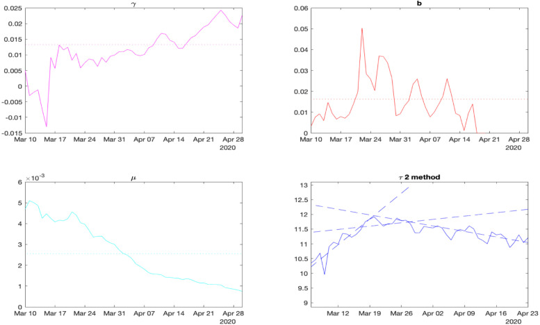
In this section, we introduce the used data together with the selected parameters, identify the parameters (as illustrated for France in Fig. 3) and simulate the interval predictor (as in Fig. 6 together with the plots of validation Fig. 7). The common parameters assigned to all countries (to simplify the analysis) are:

$$\sigma =\frac{1}{7},\kappa =0.1,$$

for chosen values of $p_Q,p_N,p_R,p_M$.5 Adjusting these values for each country improves the forecast precision, but our goal here is to illustrate the proposed method’s broad applicability for the virus propagation interval prediction.

Fig. 3.

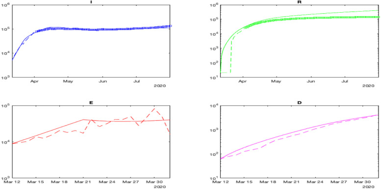
The identified parameters for France.

Fig. 6.

The results of simulation of (9) for France under $\pm 7.5\text{\%}$ variation of all parameters.

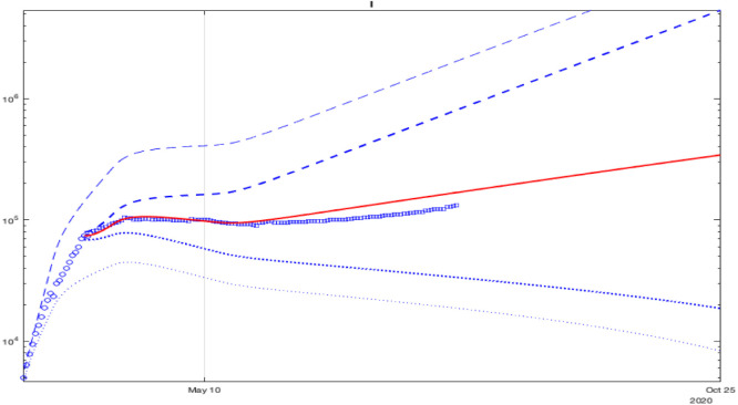
Fig. 7.

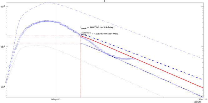
Validation of prediction of $I$ for France with $J\text{-}120$ points of data under deviations of values of all parameters.

For most countries, the first date of data acquisition is March 12th, except for Italy (March 5th), New York State (March 16th), and China (January 16th). For all eight regions, the period considered for our analysis ended on July 30th. The data available from public sources is provided in Github.

Applying the proposed procedure to the parameter identification gives the results in Table 2.

Table 2.

Parameters estimation.

Region	$\mu$	$\gamma$	$b$
France	$5.3345\times 10^{-4}$	0.0184	0.0918
Italy	$9.3987\times 10^{-4}$	0.0223	0.0159
Spain	$10.00\times 10^{-4}$	0.0275	0.1041
Germany	$8.9617\times 10^{-4}$	0.0693	0.1152
Brazil	$12.00\times 10^{-4}$	0.0579	0.1473
Russia	$8.5619\times 10^{-4}$	0.0152	0.0870
New York State	$6.5199\times 10^{-4}$	0.0271	0.0815
China	$10.40\times 10^{-4}$	0.0760	0.0238

6.1. Results of identification

For France, the obtained values ${\gamma }_k,b_k$ and ${\mu }_k$ (solid lines) together with the selected average estimates $\gamma ,b$ and $\mu$ (dot lines), and the signal $ln\left(E_t\right)$ (solid line) with approximations $a_{i}t+b_i$ (dash lines) are shown in Fig. 3. As we can conclude from these results, the identification of the value of $\gamma$ is relatively reliable and converging. The mortality rate $\mu$ follows the gravity of the outbreak (it was maximal during the most severe virus propagation at the beginning of April). Also, the value of $b$ is more complicated to estimate since it depends on all quantities (we stop the identification if $p_{t-{\tau }_p}$ and $r_{t-{\tau }_r}$ are sufficiently small to avoid very noisy results; see the missing values in the plot). Finally, delays ${\tau }_r$ and ${\tau }_p$ are noticeable from the plot, and the line approximations are reasonable (if at a stage some delay cannot be recognized, then we can use a nominal value).

6.2. Simulation and validation

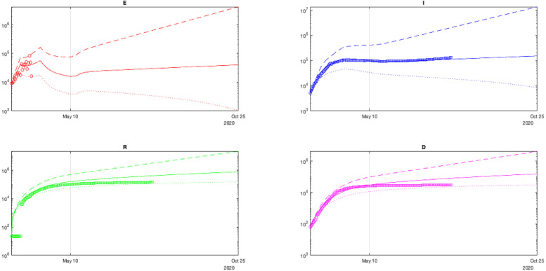
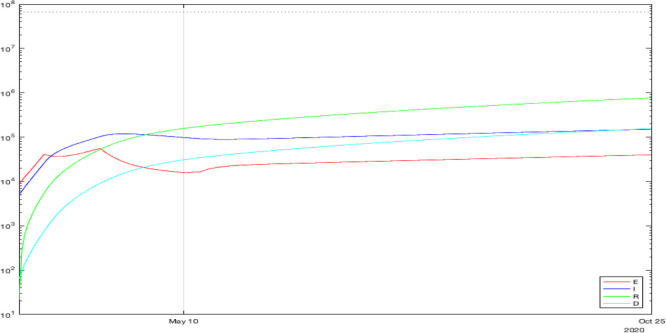
The simulation results, for France, of the model (1) with the identified parameters are given in Fig. 4 (for better visibility, all populations are plotted in the logarithmic scale), a zoomed comparison of the measured and reconstructed data is shown in Fig. 5 (as we can see, the measured data for $I$, $R$, and $D$ has a smooth shape, while the reconstructed variable $E$, also used for identification, is rather noisy). In this case, the model can approximate the virus propagation reasonably well since the identified parameters are consistent with France’s available statistics.

Fig. 4.

The results of simulation for France with identified parameters.

Fig. 5.

The results of verification with identified parameters.

The obtained curves also demonstrate the lack of efficiency of the confinement. The number of asymptomatic infectious can be reduced quickly, but symptomatic patients may persist a long time giving rise to a second wave. This conclusion might be related to the model’s probable weak validity for the decreasing phase of the outbreak.

6.3. Simulation and validation results of the interval predictor

For France, the simulation results of the interval predictor (9) with $\delta =7.5\text{\%}$ is presented in Fig. 6 (the dashed and dotted lines represent, respectively, upper and lower interval bounds, the solid lines correspond to the average behavior, the circles depict measured and reconstructed data points used for identification). The width of the predicted interval of admissible values for the state of (1) is growing, which is related with a high level of uncertainty reflected by $\delta$ and chosen for these simulations (according to Theorem 1, the dynamics of upper bounds of these variables are unstable, and the lower ones are converging to zero). For the sake of brevity, the simulation results for the remaining geographic regions are not presented here: the obtained model follows well the measured statistics for all countries and state.

As we can conclude from these curves, under sufficiently significant deviations of the parameters (which correspond to the amount and quality of data publicly available), the confinement may slow down the epidemics. The measurements are nearly included in the obtained intervals validating the prediction (the value of $\delta$ was selected to ensure this property). There are two variants of epidemic development demonstrated in these results: optimistic, which corresponds to the lower bounds of $I$ and $E$, and pessimistic presented by the respective upper bounds.

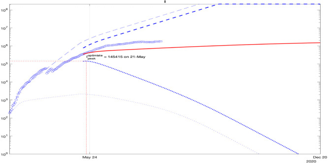
To check the prediction accuracy, we can select a part of the data for identification and another part for verification of prediction reliability. Such validation results are shown in Fig. 7, where the interval prediction for the infectious population $I$ is presented with a deviation of all parameters. As previous, blue dashed and dotted lines correspond do the upper $\overline{I}$ and the lower bounds $\underset{\_}{I}$, the bold lines are calculated using $J\text{-}1$ day initial conditions), the blue circles and squares are the measured information used for identification and validation, and the red line is the average behavior. In the plot, only the data points for $t=0,1,\dots ,J-120$ are used, shown by circles, and the interval predictor is initiated with the data for $t=J-121$. Then, square data points (which were not taken into account during identification for $t=J-120,\dots ,J$) can be compared with the predictor trajectories (bold dashed and dotted blue lines and the red one). As we can see, the points marked by squares are well included in the predicted interval, which confirms the reliability of (9) at least for $120$ days.

In general, further precision of the model and the parameters is needed. However, as a recommendation after these preliminary simulations, the preservation of the quarantine rules is desirable (the simulation clearly demonstrates the epidemics decreasing during lockdown only). The model shows a relatively low decrease in the number of infected individuals, then prolonging the isolation of the fragile part of the population, and social distancing is reasonable (it is worth noting that the value of $p_R$ is selected ad-hoc and probably too high).

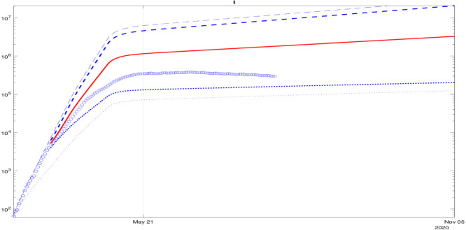
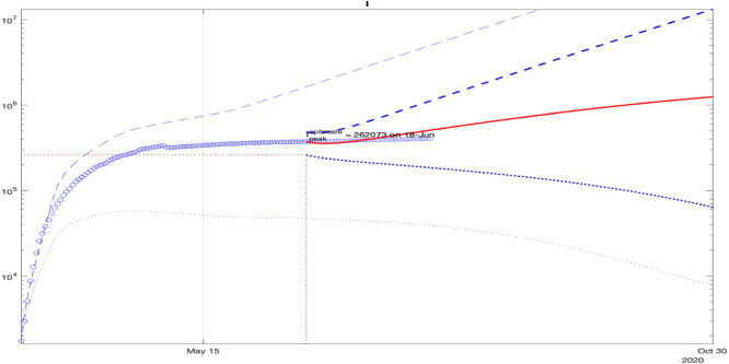
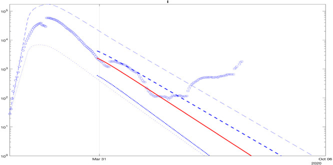
In the sequel, an analysis of the model fitting to the data for other countries and state is demonstrated in Figs. 8, 9, 10, 11, 12, 13, 14: blue dashed and dotted lines correspond to the upper $\overline{I}$ and the lower bounds $\underset{\_}{I}$ (the bold lines are calculated using the last day included in the identification data). The red line is the average, the blue circles and squares are the measured information used for identification and validation. A reasonable fit of the model to the data for Italy is demonstrated in Fig. 8. The square points belong to the middle of the predicted interval in the plot.

Fig. 8.

Validation of prediction of $I$ for Italy with $J\text{-}60$ points of data under deviations of values of all parameters.

Fig. 9.

Validation of prediction of $I$ for Spain with $J\text{-}60$ points of data under deviations of values of all parameters.

Fig. 10.

Validation of prediction of $I$ for Germany with $J\text{-}90$ points of data under deviations of values of all parameters.

Fig. 11.

Validation of prediction of $I$ for Brazil with $J\text{-}70$ points of data under deviations of values of all parameters.

Fig. 12.

Validation of prediction of $I$ for Russia with $J\text{-}120$ points of data under deviations of values of all parameters.

Fig. 13.

Validation of prediction of $I$ for NY State with $J\text{-}40$ points of data under deviations of values of all parameters.

Fig. 14.

Validation of prediction of $I$ for China with $J\text{-}120$ points of data under deviations of values of all parameters.

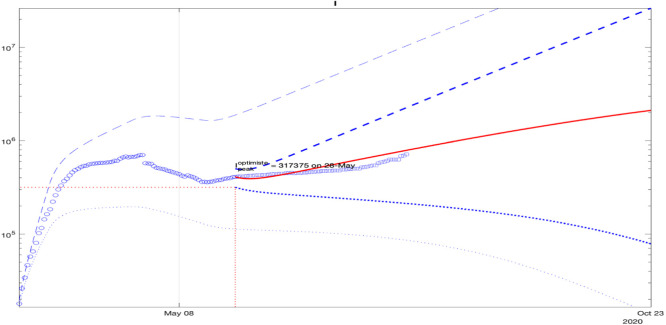
For Spain, a good fit of the model to the data is demonstrated in Fig. 9: the square points lie close to the middle of the predicted interval. For Germany, the square points in Fig. 10 are not included at the end in the predicted interval in the plot, which is related to the start of the second wave that is noticeable from the data.

For Brazil, the square points belong to the predicted interval in the plot, as shown in Fig. 11. A good fit of the model for Russia is shown in Fig. 12, where the square points belong to the lower part of the predicted interval in the plot.

A fit of the model for the NY State’s data is demonstrated in Fig. 13, where the square points belong to the middle of the predicted interval in the plot. A fit of the model to China’s data is demonstrated in Fig. 14, where the square points are not included at the end in the predicted interval in the plot, which is related to the start of the second wave that is noticeable from the data. As for Germany, this issue originated because the model parameters were identified several months before the beginning of the second wave, and in the end they lost their validity. The societal feedback and reactions also changed at that time, which is not reflected by the predictor’s inputs.

7. Conclusion

A simple new discrete-time SEIR epidemic model was identified and used to predict the quarantine’s influence on the SARS-CoV-2 virus propagation in France, Italy, Spain, Germany, Brazil, Russia, New York State, and China. An interval predictor method was developed to analyze the COVID-19 course – whose ability to take into account the sets of admissible values for initial conditions, inputs, and parameters – enlarges the prediction performance. It was demonstrated that the reliability of the interval prediction for $30-120$ days is rather good, even by such a simple model. The prediction showed that more extended confinement might be a bit more efficient, but a more strict as possible quarantine seemed to be advisable under the uncertainty level. The obtained results show that predicting the outbreak development with reasonable accuracy is possible by selecting different contact profiles between the countries’ compartments.

The eight considered countries can be divided into two groups: four European states (France, Italy, Spain, and Germany) and China, where the virus presence is already well developed with several weeks of quarantine, and two BRICS countries (Brazil and Russia) with the US, where the epidemics started later and somewhat general confinement has also been imposed later. The identified models for these groups of countries have common patterns (e.g., a significant variation of the recovery rate $\gamma$ for Brazil and Russia). Our prediction showed that in European countries, the peak of infections occurred in April–May in the optimistic scenario. Increased severity of the confinement could significantly decrease the amplitude of the peak discharging the health services load.

Machine learning tools can be further used to identify and optimize the time profile for the confinement. Another possible direction of improvement of the proposed approach is to consider a SEIR model with population separation either by age or by region (or by both), but this implies an increasing number of parameters to be identified (that can be impossible) and also needs specially structured data to be available. The introduction of delays in the proposed model dynamics to better describe the virus propagation lags between compartments is also a promising investigation area.

Declaration of Competing Interest

The authors declare that they have no known competing financial interests or personal relationships that could have appeared to influence the work reported in this paper.

References

- Aronna, M. S., & Bliman, P.-A. Interval observer for uncertain time-varying SIR-SI epidemiological model of vector-borne disease. In 2018 16th European control conference. Limassol.
- Bliman, P.-A., Efimov, D., & Ushirobira, R. (2018). A class of nonlinear adaptive observers for SIR epidemic model. In Proceedings of ECC’18, the 16th annual European control conference.
- Bohk-Ewald C., Dudel C., Myrskyla M. 2020. A demographic scaling model for estimating the total number of COVID-19 infections. medRxiv. [DOI] [PMC free article] [PubMed] [Google Scholar]
- Cantó B., Coll C., Sánchez E. Estimation of parameters in a structured SIR model. Advances in Difference Equations. 2017;2017(1):33. [Google Scholar]
- Dandekar R., Barbastathis G. 2020. Neural Network aided quarantine control model estimation of global Covid-19 spread.arXiv:2004.02752 [DOI] [PMC free article] [PubMed] [Google Scholar]
- Das S., Ghosh P., Sen B., Mukhopadhyay I. 2020. Critical community size for COVID-19 – a model based approach to provide a rationale behind the lockdown.arXiv:2004.03126 [Google Scholar]
- Degue, K. H., Efimov, D., & Iggidr, A. (2016). Interval estimation of sequestered infected erythrocytes in malaria patients. In 2016 European control conference (pp. 1141–1145).
- Degue, K. H., & Le Ny, J. (2018). An interval observer for discrete-time SEIR epidemic models. In 2018 annual american control conference (pp. 5934–5939).
- d’Onofrio A., Manfredi P., Poletti P. The interplay of public intervention and private choices in determining the outcome of vaccination programmes. PLoS One. 2012;7(10) doi: 10.1371/journal.pone.0045653. [DOI] [PMC free article] [PubMed] [Google Scholar]
- Efimov D., Raïssi T. Design of interval observers for uncertain dynamical systems. Automation and Remote Control. 2016;77(2):191–225. [Google Scholar]
- Efimov, D., & Ushirobira, R. (2020). On interval prediction of COVID-19 development in France based on a SEIR epidemic model. In Proc. IEEE conference on decision and control. Jeju Island, Korea. [DOI] [PMC free article] [PubMed]
- Ferguson N.M., Laydon D., Nedjati-Gilani G., Imai N., Ainslie K., Baguelin M., et al. WHO Collaborating Centre for Infectious Disease Modelling, MRC Centre for Global Infectious Disease Analysis, Abdul Latif Jameel Institute for Disease and Emergency Analytics Imperial College London; 2020. Impact of non-pharmaceutical interventions (NPIs) to reduce COVID-19 mortality and healthcare demand. [Google Scholar]
- Gevertz J., Greene J., Hixahuary Sanchez Tapia C., Sontag E.D. 2020. A novel COVID-19 epidemiological model with explicit susceptible and asymptomatic isolation compartments reveals unexpected consequences of timing social distancing. medRxiv. [DOI] [PMC free article] [PubMed] [Google Scholar]
- Gouzé J., Rapaport A., Hadj-Sadok M. Interval observers for uncertain biological systems. Ecological Modelling. 2000;133:46–56. [Google Scholar]
- Hu Z., Ge Q., Li S., Boerwincle E., Jin L., Xiong M. 2020. Forecasting and evaluating intervention of Covid-19 in the World. arXiv e-prints, arXiv:2003.09800. [DOI] [PMC free article] [PubMed] [Google Scholar]
- Keeling M.J., Rohani P. Princeton University Press; 2008. Modeling infectious diseases in humans and animals. [Google Scholar]
- La Salle J.P. Society for Industrial and Applied Mathematics; 1976. The stability of dynamical systems. [DOI] [Google Scholar]
- Lauer S.A., Grantz K.H., Bi Q., Jones F.K., Zheng Q., Meredith H.R., et al. The incubation period of coronavirus disease 2019 (COVID-19) from publicly reported confirmed cases: Estimation and application. Annals of Internal Medicine. 2020 doi: 10.7326/M20-0504. [DOI] [PMC free article] [PubMed] [Google Scholar]
- Leurent, E., Efimov, D., Raïssi, T., & Perruquetti, W. (2019). Interval prediction for continuous-time systems with parametric uncertainties. In Proc. IEEE conference on decision and control. Nice.
- Lopez L.R., Rodo X. 2020. A modified SEIR model to predict the COVID-19 outbreak in Spain and Italy: simulating control scenarios and multi-scale epidemics. medRxiv, arXiv:https://www.medrxiv.org/content/early/2020/04/16/2020.03.27.20045005.full.pdf. [DOI] [PMC free article] [PubMed] [Google Scholar]
- Lourenco J., Paton R., Ghafari M., Kraemer M., Thompson C., Simmonds P., et al. 2020. Fundamental principles of epidemic spread highlight the immediate need for large-scale serological surveys to assess the stage of the SARS-CoV-2 epidemic. medRxiv. [DOI] [Google Scholar]
- Magal P., Webb G. The parameter identification problem for SIR epidemic models: Identifying unreported cases. Journal of Mathematical Biology. 2018;77:1629–1648. doi: 10.1007/s00285-017-1203-9. [DOI] [PubMed] [Google Scholar]
- Magal P., Webb G. 2020. Predicting the number of reported and unreported cases for the COVID-19 epidemic in South Korea, Italy, France and Germany. medRxiv. arXiv:https://www.medrxiv.org/content/early/2020/03/24/2020.03.21.20040154.full.pdf. [DOI] [PMC free article] [PubMed] [Google Scholar]
- Maier B.F., Brockmann D. 2020. Effective containment explains sub-exponential growth in confirmed cases of recent COVID-19 outbreak in Mainland China. medRxiv. [DOI] [PMC free article] [PubMed] [Google Scholar]
- Mazenc F., Bernard O. Interval observers for linear time-invariant systems with disturbances. Automatica. 2011;47(1):140–147. [Google Scholar]
- Mazenc F., Dinh T.N., Niculescu S.I. Interval observers for discrete-time systems. International Journal of Robust and Nonlinear Control. 2014;24:2867–2890. [Google Scholar]
- Nussbaumer-Streit B., Mayr V., Dobrescu A., Chapman A., Persad E., Klerings I., et al. Quarantine alone or in combination with other public health measures to control COVID-19: A rapid review. Cochrane Database of Systematic Reviews. 2020;(4) doi: 10.1002/14651858.CD013574. [DOI] [PMC free article] [PubMed] [Google Scholar]
- Peng L., Yang W., Zhang D., Zhuge C., Hong L. 2020. Epidemic analysis of COVID-19 in China by dynamical modeling.arXiv:2002.06563 [Google Scholar]
- Raïssi T., Efimov D., Zolghadri A. Interval state estimation for a class of nonlinear systems. IEEE Transactions on Automatic Control. 2012;57(1):260–265. [Google Scholar]
- Ushirobira, R., Efimov, D., & Bliman, P. (2019). Estimating the infection rate of a SIR epidemic model via differential elimination. In 2019 18th European control conference (pp. 1170–1175).
- Wang Z., Bauch C.T., Bhattacharyya S., d’Onofrio A., Manfredi P., Perc M., et al. Statistical physics of vaccination. Physics Reports. 2016;664:1–113. [Google Scholar]
- Yang Z., Zeng Z., Wang K., Wong S.-S., Liang W., Zanin M., et al. Modified SEIR and AI prediction of the epidemics trend of COVID-19 in China under public health interventions. Journal of Thoracic Disease. 2020;12(3) doi: 10.21037/jtd.2020.02.64. [DOI] [PMC free article] [PubMed] [Google Scholar]