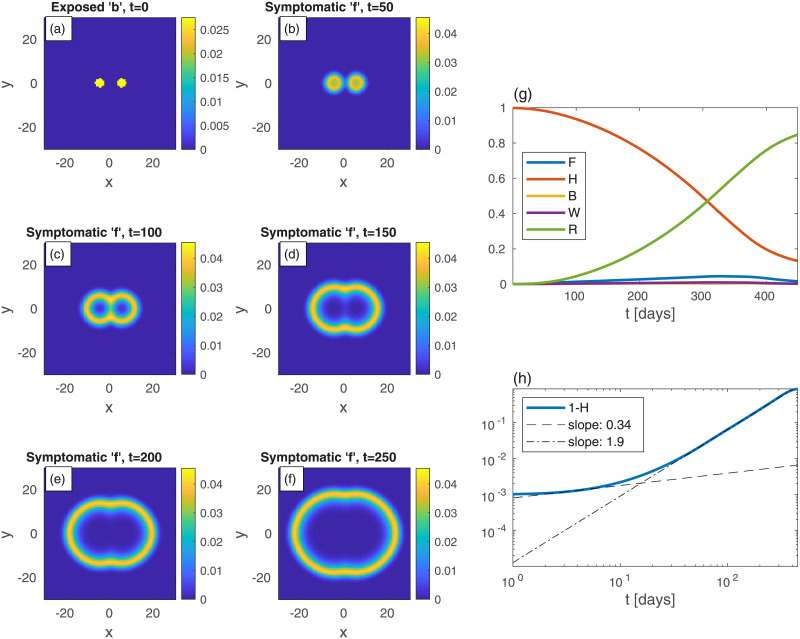
Fig 2. Time evolution of an epidemic starting from two infection centers (in this and in all other figures, t is the time in days, and x and y are the spatial Cartesian coordinates).

(a) Initial conditions of b. B—the global value of b—is the same as in Fig 1. n is uniform and all other populations are initially zero: w = f = r = 0. Panels (b)-(f) depict the spreading pattern of the symptomatic population ‘f’ as time progresses. The two circular domains grow and merge into one oval-like domain. Panel (g) shows the global sub-populations F, H, B, W, and R vs time t (in days). Panel (h) shows the cumulative fraction of infected population 1 − H vs time t in (in days) on a log-log scale. Compare to the cases of uniform (Fig 1). Dashed and dash-dotted curves in panel are linear fits at t = 3 and t = 150, respectively.