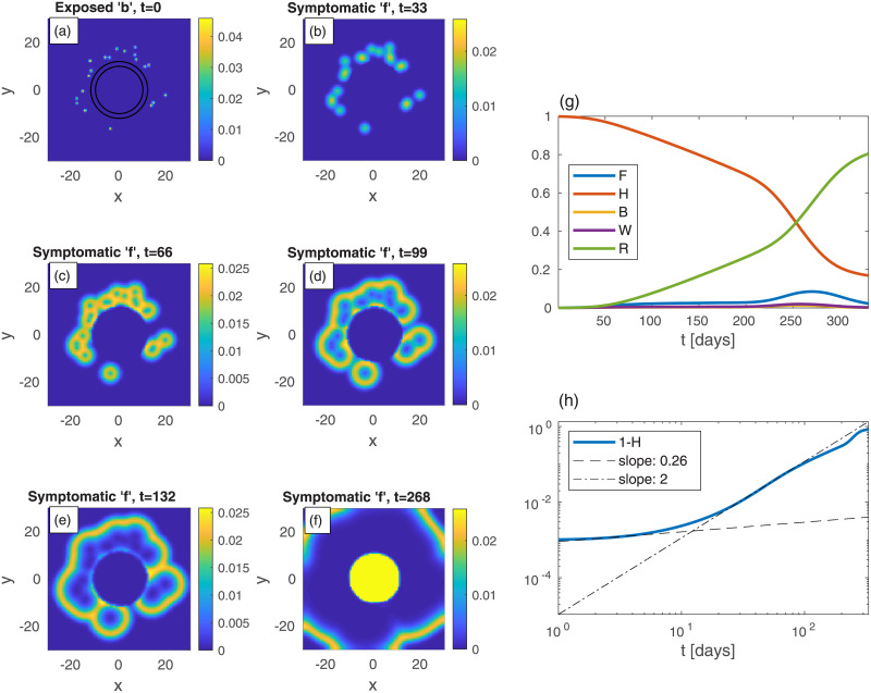
Fig 8. Belt quarantine.
Time evolution of an epidemic starting from multiple random infection centers (see panel (a)), near a city identical to that of Fig 7: n is nonuniform, and is given by n = 10a within a circle of radius 10, and n = a outside of that circle, with a taken such that the spatial average of n is 0.2; t is the time given in days, and x and y are the spatial Cartesian coordinates. The “city” is under a protective circumferential “belt”, formed by two concentric circles (radii 10 and 12), within which Dk and k are reduced to 20% of their values elsewhere. The initial (t = 0) integrated value of b is the same as in previous figures, B = 10−3. All other populations are initially zero: w = f = r = 0. Panels (b)-(f): The infection is seen to spread quickly within the external area, but penetrates very slowly into the protected region. The global sub-population fractions are shown in panels (g)-(h); F shows a very wide plateau followed by a higher peak.

