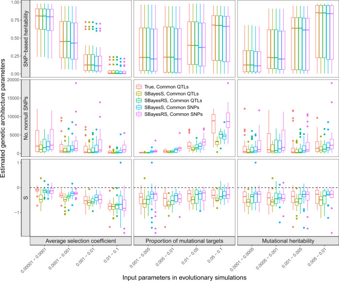
Fig. 4. Variational patterns of the estimated genetic architecture parameters under different scenarios of evolutionary simulations.

The selection coefficients followed a mixture distribution, and the Simons et al. pleiotropic model with n_t = 1 was used to generate genetic effects (see the “Methods” section). The x-axis shows the values of three input parameters in the evolutionary simulations. The y-axis shows the distribution of the genetic architecture parameter estimates, where the polygenicity parameter is represented by the number of nonnull SNPs for better benchmarking. Colours indicate the following methods: “True, Common QTLs”—parameters computed directly from the simulated genetic effects of all common causal variants; “SBayesS, Common QTLs” (or “SBayesRS, Common QTLs”)—SBayesS (or SBayesRS) estimates using the genotype data of the common causal variants, “SBayesS, Common SNPs” (or “SBayesRS, Common SNPs”)—SBayesS (or SBayesRS) estimates using the genotype data of 36k common SNPs. Each box plot shows the results of 25 independent simulation replicates. The band inside the box is the median, the bottom and top of the box are the first and third quartiles, respectively (Q1 and Q3), and the lower and upper whiskers are Q1–1.5 × IQR and Q3 + 1.5 × IQR, respectively, where IQR = Q3–Q1.