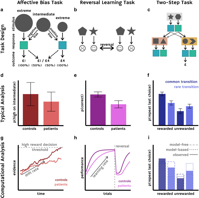
Fig. 2.

a–c The designs of the three types of cognitive task mentioned: the affective bias task, reversal learning task and two-step task. d–f Examples of how data is typically collapsed and analysed for these tasks. g–i Examples of the additional information that can be gained by taking a computational approach. a In the affective bias task, also known as the ‘ambiguous-cue interpretation task’, participants are first trained to press either the left or right button in response to the extreme stimuli (large or small circles in this example) which are 100% associated with either a £1 or £4 reward (associations counterbalanced across participants). In the test phase, during different trials, participants are shown either one of the original extreme stimuli or a novel, intermediate stimulus, to which they must respond by pressing the button associated with the stimulus they think it is closer to. On intermediate trials, there is a 50% chance of receiving a £1 or £4 reward. d Affective bias is operationalised here as the proportion of times participants press the button associated with the higher reward stimulus on intermediate stimulus trials. g An example of the drift rate, which can be estimated using a drift diffusion model (DDM), allowing us to account for participant accuracy and reaction times. In our work using this task [10], we found that patients with mood and anxiety disorders demonstrate a lower drift rate towards classifying the mid-tone as high reward. b In reversal learning tasks, participants typically choose between two stimuli on screen by pressing the corresponding button. One stimulus is associated with reward, indicated by a smiley face, and the other with punishment, indicated by a sad face. The contingencies are then reversed, so that the previously rewarded stimulus is now punished and vice versa. e The probability of participants choosing a correct (rewarded) choice. h The estimated learning rate; the shallower learning curve and greater latency before performance returns to high accuracy after a reversal is indicative of a slower learning rate in patients here. c In this example of a two-step task, participants start in one state (shown here in grey), and choose between two stimuli (star or hexagon), each of which result in a probabilistic transition (here, high probabilities are represented with a thicker arrow, and low probabilities—‘rare transitions’—with a thinner arrow) to a second-level state (either pink or orange), at which point they can choose between the two stimuli which are available to them in that state. Here, imagine that a participant chooses the star, and probabilistically moves to the orange state (on the right). They then choose the circle, which results in a reward. To obtain this reward again, the participant could perform in a ‘model-free’ way, without understanding the transitional structure of the stages, and simply choose the star again. However, this ‘model-free’ way of behaving is most likely to take them to the pink state, rather than the orange one. A ‘model-based’ choice would entail choosing the hexagon in state one, which is more likely to result in a transition to the desired orange state. When these choices are repeated over many trials, logistic regression or computational modelling can be used to demonstrate the extent to which participants behave in a ‘model-based’ way to seek out the best second state, rather than simply repeating actions which previously led to reward. f The probability of repeating the last trial, split by the outcome and transition type of the previous trial. i A computational modelling analysis of participant data (solid lines) can be used to estimate a ‘weight’ for each participant, which represents the extent to which they rely on model-based (dotted lines) and model-free (dashed lines) strategies