Seeing the wood despite the trees: Exploring human disturbance impact on plant diversity, community structure, and standing biomass in fragmented high Andean forests

Abstract

High Andean forests harbor a remarkably high biodiversity and play a key role in providing vital ecosystem services for neighboring cities and settlements. However, they are among the most fragmented and threatened ecosystems in the neotropics. To preserve their unique biodiversity, a deeper understanding of the effects of anthropogenic perturbations on them is urgently needed. Here, we characterized the plant communities of high Andean forest remnants in the hinterland of Bogotá in 32 0.04 ha plots. We assessed the woody vegetation and sampled the understory and epiphytic cover. We gathered data on compositional and structural parameters and compiled a broad array of variables related to anthropogenic disturbance, ranging from local to landscape‐wide metrics. We also assessed phylogenetic diversity and functional diversity. We employed nonmetric multidimensional scaling (NMDS) to select meaningful variables in a first step of the analysis. Then, we performed partial redundancy analysis (pRDA) and generalized linear models (GLMs) in order to test how selected environmental and anthropogenic variables are affecting the composition, diversity, and aboveground biomass of these forests. Identified woody vegetation and understory layer communities were characterized by differences in elevation, temperature, and relative humidity, but were also related to different levels of human influence. We found that the increase of human‐related disturbance resulted in less phylogenetic diversity and in the phylogenetic clustering of the woody vegetation and in lower aboveground biomass (AGB) values. As to the understory, disturbance was associated with a higher diversity, jointly with a higher phylogenetic dispersion. The most relevant disturbance predictors identified here were as follows: edge effect, proximity of cattle, minimum fragment age, and median patch size. Interestingly, AGB was efficiently predicted by the proportion of late successional species. We therefore recommend the use of AGB and abundance of late successional species as indicators of human disturbance on high Andean forests.

High Andean forests play a key role in providing ecosystem services for neighboring urban settlements. Here, we aimed to identify and understand the effects of anthropogenic perturbations on diversity, composition, and structure of plant communities, as well as aboveground biomass in high Andean forest remnants in the hinterland of Bogotá. We found that the increase of human‐related disturbance resulted in less phylogenetic diversity and in the phylogenetic clustering of the woody vegetation and in lower aboveground biomass (AGB) values. As to the understory, disturbance was associated with a higher diversity, jointly with a higher phylogenetic dispersion. Interestingly, AGB was efficiently predicted by the proportion of late successional species.

1. INTRODUCTION

High Andean tropical montane forests (herein bosques altoandinos) can be found between ca. 2,700 and 3,300 m in the Northern Andes, extending from Venezuela to Ecuador, with considerable levels of species diversity and endemism (Gentry & Ortiz, 1993; Girardin et al., 2014; Killeen et al., 2007; Still et al., 1999; Young, 1992). These forests provide vital ecosystem services to the neighboring cities and settlements, such as the regulation of water fluxes (Armenteras et al., 2003; Chaves & Arango, 1998; Linares & Ríos, 2004; Rangel, 2000) or carbon capture and storage (Brown & Kappelle, 2001; Torres et al., 2012).

Bosques altoandinos have been subjected to extensive anthropogenic transformation across their natural range. In Colombia, large portions of the forest cover were cleared during the past four centuries and turned into agricultural or residential areas, in order to satisfy the growing demand for resources of an increasing human population (Brown & Kappelle, 2001; Cavelier et al., 2001; Etter et al., 2008; Heath & Binswanger, 1996; Sánchez‐Cuervo et al., 2012; Wassenaar et al., 2007). Such a reduction of forest cover can not only lead to loss of biodiversity but also to a lower structural integrity and resilience of the remaining fragments (Mori et al., 2013). Changes in species composition also go along with shifts in functional diversity and biological interactions (Bovendorp et al., 2019; Diaz & Cabido, 2001; Flynn et al., 2011; Petchey & Gaston, 2002, 2007; Poos et al., 2009; Swenson, 2014). Eventually, this affects ecosystem services (González et al., 2011; Menon et al., 2007; Rangel, 2000; Torres et al., 2012).

In the recent past, forest cover has increasingly been monitored using remote sensing techniques. For the Colombian high Andean forests, this has shown modest signs of recovery in some areas (Calbi et al., 2020; Etter, 2002; Rubiano et al., 2017; Sánchez‐Cuervo et al., 2012; but see Anselm et al., 2018). However, remote sensing cannot detect cryptic forms of forest degradation, such as selective logging or understory grazing. Even plot‐based surveys focusing on trees may not reveal such alterations. Yet, cryptic forest degradation has significant impact on soil erosion, successional dynamics, and regeneration, since understory and epiphytic plants are major drivers of ecosystem functioning (Nilsson & Wardle, 2005). Understanding the effects of anthropogenic disturbance on all major forest components, that is, tree, shrub, understory, and epiphyte layers, is therefore essential to elaborate and implement effective strategies for the sustainable management of these forest ecosystems (Battles et al., 2001; Fahey & Puettmann, 2007; Halpern & Spies, 1995; Roberts & Gilliam, 1995). In addition, multiple predictor and response variables should be analyzed simultaneously to properly address disturbance effects within this complex environment.

One of the best areas to study the impact of human‐induced alterations on bosques altoandinos in the northern Andes is the area of Bogotá, the capital of Colombia, which is situated at approximately 2,600 m altitude. With a population of around 9 million inhabitants, Bogotá is by far the largest city in the Andean high montane forest belt, putting tremendous pressure on the surrounding ecosystems. Remnants of high Andean forests near Bogotá are mostly affected by rural activities, which include logging, fires, and agriculture, typically resulting in soil compaction, low fertility, and/or erosion (Armenteras et al., 2003; Linares & Ríos, 2004; Posada & Norden, unpublished results). Bosques altoandinos in the surroundings of Bogotá have mostly been studied using phytosociological analysis of plot inventory data (Avella et al., 2014; Cantillo Higuera & Gracia, 2013; Cleef, 1981; Cortés, 2008; Sturm & Rangel, 1985; Van der Hammen, 2008). Beyond such floristically oriented approaches, few studies have addressed the effects of disturbance on these forest ecosystems. Some preliminary research works on forest succession and regeneration were carried out as thesis works (Acuña, 2013; Restrepo Abadia, 2016). In a recent study, Rodríguez‐Alarcón et al. (2018) found a negative effect of forest fragmentation on functional diversity and aboveground biomass, a first indication that more complex parameters such as functional diversity are indeed related to ecosystem services such as carbon storage. However, studies that simultaneously consider multiple disturbance predictors and different plant communities response variables were so far lacking.

According to the available literature, the most relevant disturbance factors, which variation proved to be significantly related to differences in forest species composition or diversity metrics, are as follows: age of forest fragment (Köster et al., 2009; Laurance et al., 2006), proximity to houses or roads and people and livestock density (Ribeiro et al., 2015, 2016), edge effect, and proximity to pastures (Parra Sánchez et al., 2016; Werner & Gradstein, 2009), as well as forest cover fragmentation metrics (Fahrig, 2003; Hertzog et al., 2019; Laurance et al., 2006). Nonetheless, it has not yet been tested whether these factors would be still relevant when a larger number of variables are considered simultaneously. For this reason, we conducted a comprehensive integrated assessment of the potential effects of multiple environmental and disturbance variables on the taxonomic, phylogenetic, and functional diversity of the two main forest layers (tree layer and understory) and on epiphytes cover.

We therefore hypothesized that anthropogenic disturbance as a whole, understood as a composite variable sensu Paine et al. (1998), affects the composition, and aboveground biomass of bosques altoandinos, with impacts on community diversity metrics, that is, taxonomic, phylogenetic, and functional diversity. We also hypothesized that our comprehensive analysis would identify significant predictor and response variables other than those found in previous studies. We specifically set out to answer three questions: (a) Which environmental and disturbance variables best explain species diversity and composition of tree and understory layers? (b) What are the effects of facilitators (parameters that increase the likeliness of disturbance) and causes (direct sources) of disturbance on species diversity, phylogenetic structure, functional diversity, and aboveground biomass? (c) Which vegetation variables are best indicators of disturbance?

2. METHODS

2.1. Study area

The study area encompasses ca. 4,600 km² within the Cundiboyacense high plain in the Cordillera Oriental of Colombia, spanning peri‐urban and rural areas of the department of Cundinamarca and the administrative region of the city of Bogotá (Bogotá D.C. or Distrito Capital). The capital region is the most densely populated area of the country, with nearly 9 million inhabitants and approximately 4,500 people per km² (DANE, 2019). The climate is characterized by isothermality with an annual mean temperature of around 14°C and mean annual precipitation between 600 and 1,300 mm. There are two rainy seasons: from April to June and from September to November, with a drier and warmer season from January to March (Anselm et al., 2020; IDEAM, 2007, 2015). The topography is marked by an extended plain, situated at around 2,600 m, which hosts most of the urban and agricultural area, and steep elevation gradients including mountains of up to 4,100 m altitude. Dominant soils in the study area were classified as Andisols (IGAC, 1985; Etter, 2002; Sturm & Rangel, 1985).

Rural areas in the region are highly influenced by the adjacent city of Bogotá and contiguous suburbs. Hence, sparse remnants of original vegetation are intermixed with secondary forests (Cortés, 2008; Rubiano et al., 2017). These remnants are largely dominated, by trees and shrubs in genera such as Weinmannia, Miconia, Clusia, Hesperomeles, Clethra, Myrcianthes, Myrsine, Gaultheria and Escallonia, various genera of Lauraceae, and Cedrela montana. Hygrophytic communities with prevalence of Drimys granadensis or Hedyosmum or higher elevation heliophyte associations of Gynoxys, Diplostephium, and Vallea stipularis also form part of these ecosystems (Rangel, 2000; Sturm & Rangel, 1985; Van der Hammen, 1998). The forest patches are embedded in a landscape mosaic with cattle pastures and small‐scale cultivation of potatoes (Solanum tuberosum), green beans (Pisum sativum), and cubios (Tropaeolum tuberosum). The size of remaining forest fragments is generally small, and their regeneration is threatened by further fragmentation, invasive species, erosion (Linares & Ríos, 2004), and urbanization (Rubiano et al., 2017).

2.2. Plot setup

Due to the usually small size of forest fragments, we used a plot size of 20 × 20 m (0.04 ha) as established in the framework of the Rastrojos project (Acuña, 2013; Hurtado‐Martilletti et al., 2020; Muñoz‐Camacho et al., 2017). We complemented the data from the tree layer assessments of 20 plots obtained from the Rastrojos project with data from 12 plots set up and assessed during this study. In addition to the tree layer data, we also assessed the understory layer, and epiphyte cover in the totaling 32 plots, which are located in six administrative regions of Bogotá D.C. and Cundinamarca (Figure 1; Appendix A1). We aimed for a widely scattered position of plots in order to represent the landscape (e.g., including differently inclined slopes). Our sampling design was influenced by the distribution of available and accessible fragments. Plot locations belonged to privately owned protected areas and farms, for which we obtained the required permits of entry from the corresponding owners.

FIGURE 1.

Study area and plot locations. (a) Colombia with Bogotá Capital Department in black; (b) manually vectorized forest fragment in Guatavita; (c) Typical aspect of forest fragment in the study area: (d) Bogotá Capital Department and plot locations. Base map modified from Bing and OSM

2.3. Macro‐environmental variables

For each plot, macro‐environmental variables were compiled from different sources in QGIS 2.18.12 “Las Palmas” (QGIS Development Team, 2018). Altitude, slope, and aspect (northness and eastness) were derived from an Aster Digital elevation model of the study area; for this, ASTGTM2_N04W075, ASTGTM2_N05W075, ASTGTM2_N05W074, and ASTGTM2_N04W074 data products were retrieved from the NASA Land Processes Distributed Active Archive Center (LP DAAC; https://lpdaac.usgs.gov/tools/data‐pool, NASA/METI/AIST/Japan Spacesystems & U.S./Japan ASTER Science Team, 2009). Mean annual precipitation and mean and maximum temperature data for the period 1981–2010 were obtained from the IDEAM meteorological station closest to each plot (http://www.pronosticosyalertas.gov.co/mapas‐graficos‐tiempo‐clima/indicadores‐climatologicos). Mean population density was extracted in two buffers (radius 1 km and 5 km) around the plots from the worldpop database for South America at 1 ha resolution (https://www.worldpop.org, Sorichetta et al., 2015). A complete list of all macro‐environmental variables can be found in the Appendix A2.

2.4. Tree and shrub layer assessment

Following the protocol of Hurtado‐Martilletti et al. (2020), for every woody plant with basal diameter > 5 cm (measured at 5 cm from the ground—DAH: Diameter at “ankle” height), we recorded its DAH, DBH and visually estimated tree height, a method that proved to be quite precise for lower canopies such as the ones studied here (Silva et al., 2012). Plant material was collected and identified with the available literature (Gentry & Vasquez, 1993; Trelease & Yuncker, 1950; or webpages: https://plantasdecolombia.com), by comparison with herbarium specimens, digitized specimens available online (JBB: http://herbario.jbb.gov.co; COL: http://www.biovirtual.unal.edu.co/en/collections/search/plants), or with additional help from local experts. Specimens were deposited in the herbarium of the Jardín Botánico de Bogotá José Celestino Mutis (JBB); high‐resolution digital specimen images can be provided upon request; and a plot‐resolved list of vouchers can be found in the Appendix A3.

2.5. Understory assessment

In each 20 × 20 m plot, eight 1 × 1 m quadrants (with marked 10 cm subgrids) were placed randomly. All vascular plants, including tree seedlings, were recorded, and mean height and total cover (the sum of all individuals cover) were measured for every species in each quadrant. When available, fertile material was collected and deposited in the JBB. Additionally, cover of bare soil, leaf litter, bryophytes, lichens, and coarse woody debris was visually estimated for every quadrant.

2.6. Epiphyte cover

In each plot, we sampled 40 randomly selected trees to estimate the epiphyte cover. Categorical cover classes (ranging from 0 to 3) were assigned to each of five major epiphyte groups (bryophytes, lichens, ferns, bromeliads, and orchids), separately for trunk and canopy branches.

2.7. Functional traits and functional diversity

Three leaf functional traits (specific leaf area: SLA; leaf thickness: LT; and leaf dry matter content: LDMC) were measured for each tree species following the protocols provided by Pérez‐Harguindeguy et al., (2013). Five leaves were collected from each of up to three different individuals per species and stored in wet paper for at least 12 hr, then weighted (petiole included). LT was measured with a digital micrometer, and a digital scan of the fresh leaves was taken with a Hewlett‐Packard F4280 scanner. Leaf area was calculated with ImageJ 1.8.0 (Schneider et al., 2012). Leaves were oven‐dried at 60°C until constant weight and weighted; SLA was then calculated as one‐sided area of a fresh leaf divided by its dry mass, expressed in cm²/g. LDMC was calculated as the dry mass (mg) divided by its fully hydrated fresh mass (g), and expressed in mg/g. Additionally, wood density (WD) was obtained from Rodríguez‐Alarcón et al. (2018) and the global wood density database (Chave et al., 2009) for all tree species or, depending on availability, at genus or family level estimates, using the R package biomass (Réjou‐Méchain et al., 2018) in R Studio (R Core Team, 2018). The traits used to estimate functional diversity were SLA, LDMC, LT, WD, maximum recorded height in the plots, and life form (tree or shrub). The final trait database was completed with data from the Rastrojos project including data from published reports (Muñoz‐Camacho et al., 2017) and Posada (unpublished results).

To reduce skewness, traits were log₁₀‐transformed and computation of functional divergence, functional dispersion, functional richness, functional evenness, and Rao's quadratic entropy (FDiv, FDis, FRic, FEve and Rao's Q) was performed as indicated in Villéger et al. (2008), using the R package FD (Laliberté & Legendre, 2010; Laliberté et al., 2014). We specified “corr + lingoes, m = 3” to reduce dimensionality. Functional diversity (FD) index (Petchey & Gaston, 2002) was calculated as the total branch length of a functional dendrogram generated on a distance matrix of traits with the R function hclust, using the PD function in the R package picante (Kembel et al., 2010). We decided to compute functional diversity according to the framework proposed by Mason et al. (2005) and Villéger et al. (2008). The calculated indices provide independent information about the position and relative abundances of species in a multidimensional functional space, allowing for a more detailed examination of the mechanisms linking biodiversity to ecosystem function (Villéger et al., 2008).

2.8. Landscape metrics

A Landsat 8 raster was downloaded from the US Geological Survey and processed in QGIS with the SCP plugin (Congedo, 2016) to obtain a land cover map. Landscape metrics refer to the size, shape, configuration, number, and position of land‐use patches within a landscape and were obtained for the forest class within a 1,000 m diameter buffer zone around the plots with the LecoS plugin (Jung, 2013).

Additionally, fragments of forests were manually vectorized and the area was calculated on a prepared Bing aerial map obtained through the Openlayers plugin (see Figure 1 for an example). Distance to closest roads was calculated with the NNJoin plugin on a shapefile downloaded from the DANE Web site (2018). Also, the type of closest road (main, secondary, or track) was noted. Distances to closest houses or tracks were manually measured on the map. Presence or absence of cattle or active cultivated fields in different buffers (0 m, 50 m, 100 m, or 500 m radius) was surveyed in the field. A complete list of all landscape metrics can be found in the Appendix A2.

Minimum age of the forest cover of each plot was estimated through the visual analysis of 43 aerial pictures of the plot locations acquired from the IGAC (Instituto Geográfico Agustín Codazzi, Bogotá; a detailed list of images can be found in the Appendix A4). The pictures ranged from the year 1940 to 2000 at roughly 10‐year intervals. We searched for available pictures from our plot locations and visually located the plots on the nongeoreferenced images. For each plot, we estimated the minimum age based on the oldest documented continuous occurrence of closed forest. A further analysis of forest cover change during the last seven decades around the study plots, carried out on the same set of aerial pictures, is presented in Calbi et al. (2020).

2.9. Community composition and structural variables

Based on the available literature (Cleef, 1981; Cortés, 2008; Cuatrecasas, 1958; Sturm & Rangel, 1985; Van der Hammen, 1998), tree layer species were classified either as late successional slow‐growing, early successional fast‐growing, exotic, or “other” (see Appendix A3 for details). Additionally, understory exotic species cover was calculated. The number of species and the relative proportion of individuals (in case of trees) or the percent cover (in case of the understory) of exotic species were used as indicators of disturbance versus conservation. Variance of tree DBH and height was also computed across all trees within each plot, together with the overall number of tree individuals, stems, stems per tree, and the percentage of large trees (DBH > 30 cm). Mean understory height and cover was calculated, as well as mean epiphytes cover.

The Gini coefficient, a measure of inequality within a distribution widely used in forestry (Bourdier et al., 2016; Latham et al., 1998; Lexerød & Eid, 2006), was calculated in each plot for stem basal areas with the gini function in the R package reldist (Handcock, 2016).

2.10. Taxonomic and phylogenetic diversity

Alpha‐diversity indices (Shannon's diversity, Simpson's and Pielou's evenness) were computed for each plot with the R package vegan (Oksanen et al., 2013). Phylogenetic community structure was assessed on the basis of a published angiosperm supertree (Phylomatic tree R20120829, available at https://github.com/camwebb/tree‐of‐trees/blob/master/megatrees/R20120829.new). First, a regional pool tree was generated with the Phylomatic webtool (Webb & Donoghue, 2005), and then, branch lengths were assigned with the bladj algorithm in the software Phylocom 4.2 (Webb et al., 2008), using the wikstrom.ages file (Wikström et al., 2001). Phylogenetic diversity (PD), mean pairwise distance (MPD), mean nearest taxon distance (MNTD), and their standardized counterparts (sesPD, sesMPD, and sesMNTD) were calculated for both trees and understory in the R package picante (Kembel et al., 2010). Moreover, abundance‐weighted MPD and MNTD were calculated to account for differences in species abundance (Webb et al., 2011). Four species of the Lycopodiaceae had to be removed from the understory regional pool since the family was not included in the used supertree.

The standardized PD metrics express the difference between observed and average value in units of standard deviation (SD). Positive values indicate phylogenetic overdispersion (co‐occurring species are more distantly related than expected by chance) and negative values phylogenetic clustering (co‐occurring species are more closely related than expected by chance).

2.11. Aboveground biomass

Aboveground tree biomass was calculated with the R package biomass. Field measurements of DBH contained less than 5% missing data, so imputation of missing values was performed with the R package mice (van Buuren & Groothuis‐Oudshoorn, 2011). To balance the missing data in height measurements, a regional diameter–height model was built in biomass. Error propagation was carried out using the AGBmonteCarlo function. Wood density error (errWD) was obtained with the getWoodDensity function as prior values on the uncertainty on wood density values, obtained using the mean sd at the species, genus, and family levels of taxa having at least 10 wood density values in the Global Wood Density database (Réjou‐Méchain et al., 2017). Height error (errH) was calculated as the RSE resulting from the local height–diameter models, as in Réjou‐Méchain et al. (2017), and diameter measurements propagation error (Dpropag) was set to "chave2004," which assigns a standard important error on 5 percent of the measures, and a smaller error on 95 percent of the trees (Réjou‐Méchain et al., 2018).

Mean stand aboveground biomass (AGB) and 95% credibility interval following the error propagation were calculated with the following equation (Chave et al., 2014):

$$\text{AGB}=0.0673\ast {\left(\text{WD}\ast H\ast D^2\right)}^{0.976}$$

where AGB = aboveground biomass [kg], WD = wood density [g/cm³], H = height [m], and D = DBH [cm]. Mean AGB per tree was calculated by dividing the total AGB value of each plot by the number of tree individuals.

2.12. Data analysis

2.12.1. Drivers of species composition of tree layer and understory

Presence and abundance of all tree, shrub, and liana species were compiled for each plot. Relative abundance was calculated for tree and understory layer mean cover.

Environmental and disturbance‐related variables as well as calculated diversity and biomass metrics were assigned to one of five categories relative to disturbance: geo‐environmental = predicting, causes = predicting, facilitators (parameters that increase the likeliness of disturbance) = predicting, level (calculated complex parameters of disturbance outcomes) = response, indicators (parameters that indicate directly the degree of disturbance) = response (Appendix A2). For instance, signs of grazing or logging were considered a potential cause of disturbance, whereas the nearest distance to a road was considered a potential facilitator. Diversity indices and biomass estimation were included in the level category.

To filter for dominant variables, we first ordinated the plots based on relative species abundances using nonmetric multidimensional scaling (NMDS) in vegan, using the mds function with Bray–Curtis distances, and specifying three as maximum number of axes. Subsequently, we fitted all variables using the envfit function and examined variable ordination scores, in order to identify the variables most strongly correlated with community composition and to assess redundancy. Both predictor and response variables were included in the same analyses, and NMDS was performed separately for tree and understory layer. Second, using Sørensen distances and flexible beta (set to –0.25) as group linkage method (McCune & Mefford, 2015), cluster analysis and subsequently indicator species analysis for each cluster were carried out in PCORD 7 (McCune & Mefford, 2015), in order to further classify community types and their characteristic elements.

Following this preliminary analysis, we determined a subset of variables that correlated with the main axes above a given threshold (R _sq > 0.35; Table 1) and performed either Kruskal–Wallis or parametric ANOVA, depending on the determined conditional distribution, using the clusters as independent variables and the filtered subsets of variables as response variables.

TABLE 1.

Variables (only predictors retained) correlating with axes above R _Sq > 0.35 for trees and understory NMDS

	Variable	R sq	p
Trees	elev	0.84	0.001
	rel_hum	0.81	0.001
	like_adjacencies	0.72	0.001
	splitting_index	0.71	0.001
	patch_cohesion_index	0.68	0.001
	logg	0.63	0.001
	greatest_patch	0.63	0.001
	largest_patch_index	0.62	0.001
	land_cover	0.61	0.001
	landscape_porportion	0.61	0.001
	overall_core	0.59	0.001
	mean_T	0.54	0.001
	landscape_shannon	0.53	0.001
	effective_meshsize	0.52	0.002
	landscape_division	0.52	0.002
	cult_100	0.49	0.001
	cattle	0.49	0.001
	landscape_simpson	0.45	0.003
	cattle_100	0.42	0.003
	age	0.41	0.004
	cattle_50m	0.39	0.006
	road_dist	0.36	0.001
Understory	elev	0.74	0.001
	fragment	0.62	0.001
	overall_core	0.58	0.001
	nn_distance	0.57	0.001
	road_dist	0.55	0.001
	edge_density	0.55	0.001
	edge_lenght	0.55	0.001
	m_DBH	0.54	0.001
	like_adjacencies	0.53	0.001
	landscape_pielou	0.53	0.001
	people_density_1km	0.49	0.001
	landscape_simpson	0.49	0.001
	mAGBT	0.48	0.001
	people_density_5km	0.45	0.001
	effective_meshsize	0.43	0.001
	landscape_division	0.43	0.001
	landscape_shannon	0.43	0.001
	n_stems	0.43	0.001
	land_cover	0.41	0.002
	landscape_porportion	0.41	0.002
	n_trees	0.40	0.001
	cult_500	0.40	0.001
	mean_H	0.39	0.001
	greatest_patch	0.38	0.003
	largest_patch_index	0.38	0.003
	mean_patch	0.38	0.001
	age	0.36	0.001
	cattle_100	0.36	0.002

To verify the presence of spatial autocorrelation in our predictors and responses, we calculated a geographical distance matrix between study plots and performed Moran's I test for all calculated variables. We detected spatial autocorrelation for 24 predictors, but none in our response variables (i.e., diversity metrics).

Finally, partial redundancy analysis (pRDA) was performed in vegan, separately for tree and understory layer. To take into account spatial autocorrelation, we fitted a pRDA specifying “locality” as condition, to be able to rule out locality effect on the ordination. The “condition” argument thereby defines partial terms that are fitted before other constraints and can be used to remove the effects of background variables, and their contribution to decomposing inertia (variance) is reported separately (Oksanen et al., 2013). Additionally, we performed Hellinger transformation of our community data as recommended by Legendre and Gallagher (2001). We further selected predictors from the set obtained with the NMDS screening, by checking for correlation (r > 0.7), performing Variance Inflation Factor (VIF) analysis (setting the threshold to 10), and then using the vegan ordistep function which performs automatic stepwise model building for constrained ordination methods (Oksanen et al., 2013).

2.12.2. General linearized models between main causes and facilitators of disturbance and main response variables

To select meaningful variables to fit our GLMs, we inspected the NMDS and pRDA graph and selected a set of uncorrelated response variables based on the direction of the arrows in the graphs. We then compiled a set of predictor variables that correlated with each selected response and checked for correlation within each set, removing one of the elements in pairs with r > 0.7. In parallel, we merged all predictor sets and removed highly correlated and spatially autocorrelated variables. Once a set of consensus predictors was obtained, we conducted a VIF analysis (setting the threshold to 10) and obtained a reduced set of primary and secondary predictors (Table 2). We thus reduced the pool of geo‐environmental variables to four, that of causes to four, and that of facilitators to seven. In addition, we selected response variables for level, including diversity metrics and indicators.

TABLE 2.

Retained predictors for GLMs building

Predictors		Responses
Geo‐environmental		Tree layer diversity
north	northness	TSR	tree species richness
slope	slope	TPielou	tree Pielou's evenness
mean_prec	mean annual precipitation	Tshann	tree Shannon's diversity
mean_T	mean annual temperature	TsesPD	tree standardized phylogenetic diversity
Causes		TsesMPDABU	abundance‐weighted trees standardized mean pairwise distance
cult_50m	cultivated fields in 50 m buffer	TsesMNTDABU	abundance‐weighted trees standardized mean nearest taxon distance
cattle	presence of cattle	FDis	Functional Dispersion
logg	logging signs	Feve	Functional Evenness
protected	pretected status	FDiv	Functional Divergence
Facilitators		FRic	Functional Richness
path_dist	distance from closest path	AGBplot	plot above‐ground biomass
house_dist	distance from closest house	Understory diversity
track_dist	distance to closest track	HSR	understory species richness
edge	the plot is located at the edge of the fragment	Hpielou	understory Pielou's evenness
age	minimum age of the plot	Hshann	understory Shannon's diversity index
cattle_100	presence of cattle in 100 m buffer	HsesPD	understory standardized phylogenetic diversity
median_patch	median forest patch size in 1 km buffer	HsesMPDABU	abundance‐weighted understory standardized mean pairwise distances
Indicators		HsesMNTDABU	abundance‐weighted understory standardized mean nearest taxon distances
n_inv_sp_T	number of invasive species of trees
n_FST_sp_T	number of fast‐growing species of trees
n_FST_ind_T	number of fast‐growing species of trees individuals
%_n_CON_sp_T	% of species of trees associated with conserved forests
Level
n_large_trees	number of trees with DBH > 30 cm
n_stems	number of stems
n_trees	number of trees
n_sp > 10DBH	number of species with DBH > 10 cm
Tree layer diversity
FDiv	Functional divergence
FRic	Functional richness
FDis	Functional dispersion
FEve	Functional evenness
Tshann	Trees Shannon diversity index
TsesMPD	Trees standardized mean pair distance
TsesMPDABU	Abundance‐weighted trees standardized mean pairwise distance
TMNTDABU	Abundance‐weighted trees standardized mean nearest taxon distance
AGBplot	plot aboveground biomass

Predictor categories refer to the groups of predictor variables categorized in (Appendix A2).

For each selected response, we identified the best conditional distribution and then performed automated selection of the optimal Generalized Linear Model (GLM) with the regsubsets function in the leaps package (Lumley & Lumley, 2013), unifying all groups of predictor variables. We specified a maximum number of predictors of four. Predictors were scaled, and a “log” link was specified in the family argument.

Thus, our GLMs related separately number of species (trees and understory), species diversity (Shannon and Pielou's indices for trees and understory), abundance‐weighted phylogenetic diversity and structure (trees sesPD, sesMPDABU, sesMNTDABU; understory sesPD, sesMPDABU, sesMNTDABU), functional diversity (FDiv, FRic, FEve, FDis), and aboveground biomass (AGBplot) as response variables with selected explanatory variables among each group of predictors (geo‐environmental causes and facilitators).

Second, we performed automated selection of the optimal GLMs with AGB, understory number of species, understory Shannon's and Pielou's indices, understory phylogenetic diversity and structure, as response variables and tree diversity indices, level and indicators of disturbance as sets of secondary predictor variables.

3. RESULTS

3.1. Plot‐based species inventory of tree and understory layers

3.1.1. Tree layer

We recorded 9,841 tree individuals belonging to 98 taxa. From these, 89 were identified to species level, six to genus, one to family, and two lianas remained unidentified due to lack of leaves, flowers, or fruits required for identification (see the Appendix A3 for the complete list of species and collected herbarium vouchers). Identified taxa belonged to 64 genera and 41 families. The only conifer recorded in the study area was Podocarpus oleifolia, and the only tree fern was Blechnum schomburgkii.

Asteraceae (14 species), Melastomataceae, Ericaceae, Primulaceae (with 6 species each), Lauraceae, and Rosaceae (5) were found to be the most diverse families in the study area. Miconia squamulosa (1,194 individuals) and Cavendishia bracteata (1,130) were the most abundant species across the study area, followed by Weinmannia tomentosa (805) and Daphnopsis caracasana (522).

3.1.2. Understory layer

Overall, 326 understory taxa were recorded, with 266 of them identified to species level, 59 to genus, and one to family level (Appendix A3). Identified taxa belonged to 174 genera and 82 families. Orchidaceae (41 species), Asteraceae (38), and Polypodiaceae (16) were the most diverse families, followed by Piperaceae (13), Bromeliaceae (12), Melastomataceae (11), Dryopteridaceae (10), Ericaceae (9), and Rosaceae (9). Dryopteridaceae, Orchidaceae, Poaceae, Blechnaceae, and Bromeliaceae were the most abundant families.

3.2. Plot‐based community ordination (NMDS, cluster analysis and Kruskal–Wallis test/ANOVA)

3.2.1. Tree layer

For the 3D ordination solution, we obtained a final stress value of 0.1160879 after 206 iterations. Visual interpretation of the NMDS graph led to the identification of three main groups. The subsequent cluster analysis revealed three additional groups, which showed deep divergence in the dendrogram (nodes at less than 50% remaining information), totaling six groups/clusters, which were used for the indicator species analysis (see Appendix A5 for further details on the indicator species analysis results).

The NMDS graph (Appendix A6) showed numerous statistically significant axis correlations of environmental variables including elevation, relative humidity, and mean temperature, while the Kruskal–Wallis test and parametric ANOVA showed that floristic differences among all groups were related to elevation (chi‐sq = 25.94, p = .0009), mean temperature (chi‐sq = 20.99, p = .0008), relative humidity (chi‐sq = 25.71, p = .0001), presence of logging (chi‐sq = 17.57, p = .0035), presence of cattle (chi‐sq = 21.05, p = .0008), presence of cattle in a 50 m buffer (chi‐sq = 15.90, p = .0071), presence of cultivated fields in a 100 m buffer (chi‐sq = 23.94, p = .0002), Shannon's landscape diversity (F = 5.58, p = .0013), like adjacencies (chi‐sq = 18.37, p = .0025), distance to roads (chi‐sq = 19.45, p = .0016), and minimum age of the fragment (chi‐sq = 11.95, p = .0355).

The resulting NMDS graphs highlighted some interesting patterns. The NMDS graph of axis 1 versus 2 depicted the variables linked to aboveground biomass (AGB), percentage of late successional species, DBH, height and minimum age on the right hand side, opposite to the variables linked to the number of fast‐growing species of trees, mean exotic species cover in the understory, or to the number of trees and the number of stems in the plots (inverse correlation). In the same plot, the AGB showed high positive correlation with distances to roads, lichen cover in the canopy and mosses cover on the soil and inverse correlation with functional diversity, and Gini coefficient. Moreover, trees abundance‐weighted mean nearest taxon distance (TMNTDABU) lied opposite to the indicators of fragmentation. A complete table of NMDS variable correlation filtered through species abundance can be found in Appendix A7.

3.2.2. Understory layer

For the 3D ordination solution, we obtained a final stress value of 0.1514607 after 20 iterations. Visual grouping within the NMDS graph was not feasible (Appendix A8). The cluster analysis identified five main groups/clusters selecting nodes at less than 20% remaining information. Indicator species analysis did not clearly separate the plot localities from each other (Appendix A5).

Kruskal–Wallis test and parametric ANOVA showed that floristic differences among all groups were related to elevation (chi‐sq = 24.06, p = .0001), distance to roads (chi‐sq = 14.23, p = .0066), edge density (F = 4.93, p = .004), presence of cultivated fields in a 100 m buffer (chi‐sq = 23.93, p = .0002), mean tree AGB (chi‐sq = 13.69, p = .01774), Shannon's landscape diversity (F = 3.04, p = .0343), people density in a 5 km buffer (chi‐sq = 15.88, p = .0032), and presence of cultivated fields in a 500 m buffer (chi‐sq = 8.35, p = .0797).

In the understory, elevation again was the most correlated environmental variable with species abundances (see Appendix A7 for details on variables correlation with NMDS axis). In the NDMS graph of axis 1 versus 2, the indicators of fragmentation, together with the presence of cattle and cultivated fields in the vicinity, were located opposite to the indicators of continuous forest cover and most of trees diversity metrics. AGB correlated directly with number of late successional species and distance to paths and tracks, and inversely with the number of fast‐growing species of trees and exotic understory species. Most of understory diversity metrics pointed toward the lower part of the graphs, together with fragmentation indicators and exotic species cover in the understory, number of trees, stems, and fast‐growing species of trees. Understory phylogenetic mean pairwise distances were correlated with AGB.

3.3. pRDA

3.3.1. Tree layer

From the set of 25 variables with R _sq > 0.35 (Table 1), after testing for redundancy, we limited our analysis to a subset of 10 variables: elevation, presence of logging, Shannon's landscape diversity, mean temperature, presence of cattle, presence of cultivated fields in a 100 m buffer, minimum fragment age, distance to roads, and presence of cattle in a 50 m buffer. The ordistep function selected seven of these: elevation, presence of logging, Shannon's landscape diversity, mean temperature, presence of cattle, minimum fragment age, and distance to roads.

The pRDA had an R _sq of 0.23 and adjusted R _sq of 0.17. The proportional conditional explained variance was 0.45, while the constrained explained variance was 0.24. The unconstrained explained variance was 0.31. Presence of cattle and lower distances to roads were associated with tree layer group 1 which was also positively correlated with Shannon's landscape diversity and negatively with elevation. Group 4 was defined by lower values of Shannon's landscape diversity and was positively correlated with minimum fragment age. Group 5 had some degree of negative correlation with minimum fragment age. Group 6 had an inverse correlation with elevation and minimum fragment age, and was associated with signs of logging, higher Shannon's landscape diversity, and absence of cattle. Groups 2 and 3 were not characterized by any particular association with the ordination variables (Figure 2).

FIGURE 2.

pRDA and Cluster analysis convex hulls of the tree layer. RDA graphs with convex hull volumes of tree layer groups for axis 1–2 (a), 2–3 (b), and 1–3 (c). (d) cluster dendrogram of plots species communities. Group 1 had Myrcianthes leucoxyla, Viburnum triphyllum, and Miconia elaeoides as statistically significant indicator species and comprised plots from Torca, Tabio, and Guatavita. Group 2 was characterized by Monticalia pulchella, Macleania rupestris, and Ilex kunthiana, and comprised plots exclusively from Pasquilla. Group 3 had Gaultheria anastomosans, Ageratina glyptophlebia, Buquetia glutinosa, Ageratina boyacensis, Berberis glauca, and Vaccinium floribundum as statistically significant indicator species, and comprised exclusively plots form Sumapaz. Group 4 was characterized by Myrsine coriacea and Clusia multiflora and included plots from Torca and Guasca. Group 5 included Cavendishia bracteata, Diplostephium rosmarinifolium, Gaiadendron punctatum, and Ulex europaeus, and comprised only plots from Guasca. Group 6 had Varronia cylindrostachia and Myrsine guianensis and included plots from Tabio and from Torca. For detailed IVI values and relative p‐values refer to the Appendix A5

3.3.2. Understory layer

From the set of 38 variables with R _sq > 0.35 (Table 1), after the assessment of redundancy, we limited our analysis to a subset of 10: elevation, number of trees, edge density, Shannon's landscape diversity, mean tree aboveground biomass (mAGBT), presence of cultivated fields in a 500 m buffer, minimum fragment age, distance to roads, people density in a 5 km buffer, and fragment size. The ordistep function selected seven of these: elevation, edge density, Shannon's landscape diversity, mAGBT, presence of cultivated fields in a 500 m buffer, distance to roads, and people density in a 5 km buffer.

The pRDA had an R _sq of 0.26 and adjusted R _sq of 0.11. The proportional conditional explained variance was 0.29, while the constrained explained variance was 0.26. The unconstrained was 0.45.

The results of the pRDA indicated that group 1 was characterized by higher values of Shannon's landscape diversity, lower values for distance from roads, lower elevation, and lower edge density. In contrast with that, group 2 was linked with higher values for distance from roads, higher elevation, lower Shannon's landscape diversity, absence of cultivated fields in a 500 m buffer, and lower population density. Group 3 had lower values of mean tree biomass and higher values of population density. Group 5 was associated with lower values of mean tree biomass. Group 4 was not characterized by any particular association with the ordination variables (Figure 3).

FIGURE 3.

pRDA and Cluster analysis convex hulls of the understory. RDA graphs with convex hull volumes of understory groups for axis 1–2 (a), 2–3 (b), and 1–3 (c). (d) cluster dendrogram of plots species communities. The first group had Oreopanax incisus and Passiflora bogotensis as indicator species (Appendix A5) and included plots from Torca and Tabio. The second group had Elaphoglossum lingua as indicator species, including plots form Pasquilla, Guasca, and Torca. The third group had Monnina aestuans, Peperomia rotundata, and Nertera granadensis among higher valued indicator species. It included only two plots, one from Sumapaz and one from Pasquilla. The fourth group had Greigia stenolepis and Rubus acanthophyllos among indicator species and comprised plots from Sumapaz and Guasca. The last group had Ageratina asclepiadea as indicator species and comprised plots from Guatavita, Guasca, and Tabio. For detailed IVI values and relative p‐values refer to the Appendix A5

3.4. Generalized linear models

A total of 15 primary predictors, 17 secondary predictors, and 17 responses were retained for GLM building (Table 2). Significant variables in GLMs with either a good fit (McFadden R _sq > 0.2) or a high Nagelkerke value (variance explained > 0.50) are reported below (Tables 3, 4 and 5). A complete table of all fitted GLMs is provided in Table S1. None of the variables associated with epiphytes cover was retained through the variable selection process and analysis.

TABLE 3.

GLMs of predictors versus responses, showing only GLMs with a good fit

Response	Best model	Variable	Coefficients				Pseudo R 2
			Estimate	SE	t value	p value (>|t|)	McFadden	Nagelkerke
Tshann	Tshann ~ slope+mean_T + house_dist+cult_50m	(Intercept)	0.70361	0.02540	27.699	<2e−16	0.752990	0.814632
		slope	−0.08664	0.02698	−3.211	.0034
		mean_T	−0.02686	0.02873	−0.935	.3580
		house_dist	−0.04705	0.02583	−1.822	.0796
		cult_50m	−0.04004	0.02870	−1.395	.1744
Hshann	Hshann ~ track_dist+mean_prec + age+house_dist	(Intercept)	0.89579	0.02215	40.441	<2e−16	0.669964	0.759986
		track_dist	0.06937	0.02916	2.379	.024680
		mean_prec	0.08776	0.02867	3.061	.004944
		age	−0.10445	0.02380	−4.389	.000157
		house_dist	−0.03438	0.02257	−1.523	.139413
AGB	AGBplot ~ slope+age + cattle+cult_50m	(Intercept)	1.7145	0.07224	23.734	<2e−16	0.150415	0.525516
		slope	−0.17248	0.07773	−2.219	.035092
		age	0.31665	0.07803	4.058	.000379
		cattle	0.23182	0.09783	2.370	.025207
		cult_50m	−0.23070	0.09631	−2.395	.023807

Predictor categories refer to the groups of predictor variables categorized in the Appendix A2.

TABLE 4.

GLMs of secondary predictors versus responses, showing only GLMs with a good fit

Response	Best model	Variable	Coefficients				Pseudo R 2
			Estimate	SE	t value	p value (>|t|)	McFadden	Nagelkerke
Hshann	Hshann ~ FDis+FRic + n_stems+n_inv_sp_T	(Intercept)	0.89802	0.02507	35.825	<2e−16	0.370602	0.474078
		FDis	−0.07597	0.03485	−2.180	.0382
		FRic	0.07827	0.03082	2.540	.0172
		n_stems	0.03100	0.02455	1.262	.2176
		n_inv_sp_T	−0.04740	0.02916	−1.626	.1156
HsesMPDABU	HsesMPDABU ~ FDiv+FRic + n_sp.10DBH + TsesMPDABU	(Intercept)	0.82655	0.07123	11.605	5.32e−12	0.261149	0.581732
		FDiv	0.24527	0.08248	2.974	.00613
		FRic	−0.26250	0.08501	−3.088	.00463
		n_sp.10DBH	0.12922	0.07900	1.636	.11351
		TsesMPDABU	0.15706	0.05962	2.634	.01380
AGB	AGBplot ~ TsesMPD+n_large_trees + n_trees+%n_CON_sp_T	(Intercept)	1.7140	0.07467	22.955	<2e−16	0.151863	0.528924
		TsesMPD	−0.06882	0.11824	−0.582	.56535
		n_large_trees	0.36350	0.11200	3.246	.00312
		n_trees	0.22454	0.10409	2.157	.04005
		%n_CON_sp_T	0.29929	0.11420	2.621	.01423

Predictor categories refer to the groups of predictor variables categorized in the Appendix A2.

TABLE 5.

GLMs variables relationships: + indicates a positive relationship and − indicates a negative relationship. Higlighted cells represent GLMs with a good fit

	TSR	Tshann	Tpielou	TsesPD	TsesMPDABU	TsesMNTDABU	HSR	Hshann	Hpielou	HsesPD	HsesMNTDABU	HsesMPDABU	FDis	FDiv	FEve	FRic	AGB
mean_T			−							−							−
mean_prec								+
north	+
slope	−	−	−			−						−	−			−	−
logg	−								+						−
cattle																	+
cult_50m						−	−				+						−
protected				−							−
edge										−	−	+	+	−		−
house_dist	−
cattle_100					−	−					+
median_patch							−
age								−	−								+
track_dist								+		−
n.sp_10DBH											+
n_trees											+						+
n_large_trees																	+
%n_CON_sp_T																	+
n_FST_ind_T										+	+
n_stems									+
FDiv							+					+
FRic								+		+	−	−
FDis								−		−
TsesMPDABU										+		+
TsesMPD									+

Tree layer Shannon's diversity decreased with slope. Understory Shannon's diversity increased with distance to tracks, mean precipitation, and tree layer functional richness (FRic), but decreased with minimum age and functional dispersion (FDis). Understory abundance‐weighted phylogenetic mean pairwise distances (HsesMPDABU) increased with functional divergence (FDiv) and tree layer abundance‐weighted phylogenetic mean pairwise distances (TsesMPDABU) and decreased with FRic. Aboveground biomass (AGB) increased with increasing minimum age of the plot and presence of cattle within the plot, and decreased with slope and proximity of cultivated fields. AGB also increased with the number of trees and large trees and with the proportion of late successional species of tree.

3.4.1. Other general trends (from models without a good fit)

Among environmental predictors, slope had a negative effect on FDis, FRic, HsesMPDABU, tree layer species richness (TSR), tree layer Pielou's evenness (Tpielou), tree layer abundance‐weighted mean phylogenetic nearest neighbor distance (TsesMNTDABU). Mean temperature had a negative effect on understory phylogenetic diversity (HsesPD) and Tpielou. Northness had a positive effect on TSR. Among the causes predictors, logging had negative effect on functional evenness (FEve) and TSR, and a positive effect on understory layer Pielou's evenness (Hpielou). The presence of cultivated fields in the immediate surrounding of plots (50 m) had a negative effect on HSR and TsesMNTDABU and a positive effect on understory abundance‐weighted mean phylogenetic nearest neighbor distance (HsesMNTDABU). Protection status had a negative effect on HsesMNTDABU and tree layer phylogenetic diversity (TsesPD). As to the facilitators, the edge effect was linked with higher values of FDis and HsesMPDABU, and lower values of HsesMNTDABU, HsesPD, FDiv, and FRic. Increasing distance from houses had a negative effect on TSR, while increasing distance from tracks had negative effect on HsesPD. The presence of cattle in a 100 m buffer was linked to higher values of HsesMNTDABU, and lower values of tree layer abundance‐weighted mean phylogenetic pairwise distance (TsesMPDABU) and TsesMNTDABU. Median patch size had negative effect on HSR. Increasing minimum fragment age had a negative effect on HPielou. Coming to the secondary predictors, the number of species with DBH > 10 cm and the number of trees had positive effect on HsesMNTDABU. The number of fast‐growing trees species individuals had a positive effect on HsesMNTDABU and HsesPD. The number of stems had a positive effect on Hpielou. FDiv had a positive effect on HSR. FRic had negative effect on HsesMNTDABU and positive on HsesPD. FDis had a negative effect on HsesPD. Finally, TsesMPDABU had positive effect on HsesPD and TsesMPD had positive effect on Hpielou.

4. DISCUSSION

Pressure of urbanization on natural environments and its consequences has been the subject of numerous studies. However, high Andean forests (bosques altoandinos) have rarely been investigated in this context. Our study is the first to analyze the role of multiple factors in shaping environmental impact on these forests through urbanization and associated factors in the metropolitan area of Bogotá. However, we are aware of the limitations of this research, which is of rather explorative character and based on data from an area of in total 1.28 ha only. Our sampling design reflects the hurdles of working in a mixed urban–rural matrix, mostly privately owned. Also, having a limited number of plots, we decided to put a stronger emphasis on the variables filtering, to drastically reduce the number of tested hypotheses. Nevertheless, the studied forest fragments belong to several of the localities harboring the highest forest cover within the Capital District and we find the types of high Andean forests covered here to be representative for the hinterland of Bogotá.

Using the composition of natural vegetation as a benchmark, our study plots were dominated by Melastomataceae, Ericaceae, and Asteraceae in the tree layer, which is in accordance with previous work (Cuatrecasas, 1934, 1958; Franco et al., 2010; Torres & Marina, 2016). Bromeliaceae and Orchidaceae were the most diverse families in the understory, coinciding with reports by Cuatrecasas (1934, 1958) and Rangel et al. (2008). Notably, with the exception of Rangel et al. (2008), no recent inventories of the understory were undertaken in the target area prior to this study. The fact that many epiphytic species were found terrestrial in the understory may be due to certain favorable environmental conditions, such as low incidence of light, high humidity, and lower influence of wind than in the canopy (Krömer et al., 2007).

Overall tree species richness of the total area assessed (98) was similar to the 90 taxa reported by Rodríguez‐Alarcón et al. (2018) for an ecologically similar study area near Bogotá. Van der Hammen (1998) reported 50–60 species for 500 m² plots of high Andean forest in the watershed of the Rio Bogotá, 20–30 of which belonged to trees and shrubs. Our own tree species count ranged between 10 and 24, with an average of 16, per 400 m² plot, and Shannon's tree diversity varied between 1.05 and 2.6. Overall, these figures also compare well to those reported for high Andean forest ecosystems (2,300–2,900 m) in Southern Ecuador by Cabrera et al. (2019), who used a higher DBH threshold (10 cm) and obtained about 21 tree species and an average value of 2.44 for Shannon's diversity.

Thus far, only few published studies exist for the target area that aimed at characterizing the various communities of bosques altoandinos in terms of species composition. Using a phytosociological approach, Cortés et al. (1999) and Cortés (2008) described the Myrcianthes leucoxyla‐Miconia squamulosa community for the internal slopes of the Rio Bogotá watershed, characterized by scarce humidity and low precipitation, with high abundance of Oreopanax incisus and conspicuous lianas in the understory. This community corresponds to our tree clusters 1 and 6 and understory clusters 1 and 5. The pRDA further revealed a lower elevation, higher Shannon's landscape diversity, lower minimum fragment age, presence of logging and lower distance to roads as characteristic for this community, supporting the notion that it represents secondary forest, probably developing on patches of abandoned agricultural areas on the slopes surrounding cultivated and farmed plains (Cortés, 2008). Understory cluster 5 was generally found at medium elevations, on small high plains, with a drier climate (Cortés, 2008; Cortés et al., 1999), and in forest patches with generally low values of aboveground biomass.

The Drimys granadensis‐Weinmannia tomentosa community is a second bosque altoandino subtype (Vargas & Zuluaga, 1980), corresponding to our tree clusters 2 and 4. Cluster 2 is similar to the Criotoniopsis bogotana‐Weinmannia tomentosa forest subtypes described for elevations between 3,100 and 3,300 m (Cortés, 2008), whereas cluster 4 is found at the slopes and peaks of the watershed of the Río Bogotá between 2,700 and 3,200 m (Cortés, 2008). According to Cortés (2008) and Luteyn (2002), the presence of Macleania rupestris in the lower canopy of these communities points toward recent human intervention. This association is known to prefer humid, cold climates and steep grounds; according to our field observations, it is also associated with high lichen and moss cover in the canopy, which prosper in such a relatively high humidity (Batke et al., 2015; Munzi et al., 2014; Wolf, 1993). As shown in the pRDA ordination, it is also linked to low Shannon's landscape diversity, and higher minimum fragment age, probably representing secondary forest fragments approaching the structure of natural forest communities.

Our tree clusters 3 and 5 did not correspond to previously described communities. Cluster 3 was restricted to bosques altoandinos near Sumapaz, the largest known paramo on Earth. Characteristic elements of this cluster are families of high elevations such as Asteraceae and Ericaceae (Bach et al., 2007; Cuatrecasas, 1958; Sturm & Rangel, 1985), also typically found in areas subjected to fires or selective logging (Cuatrecasas, 1958). The latter notion is supported by the observed presence of both cattle and cultivated fields in the immediate surrounding, by a high Shannon's landscape diversity, and by the presence of logging, indicating recent and ongoing intervention in the area. Nonetheless, full‐grown individuals of Weinmannia fagaroides and Polylepis quadrijuga were found in two of the plots of this cluster, together with some young individuals of Podocarpus oleifolia and Berberis glauca abundant in the lower canopy, and a dense cover of mosses and ferns, which suggests that some small “islands” of mature forest elements were able to persist within the disturbed, secondary forest matrix. Understory cluster 3 did not fit any previously described communities either, but the indicator species of this cluster are known to be either dispersed by birds, for example, Monnina aestuans (Romero, 2002) and Nertera granadensis (Vargas‐Ríos, 1997), or by small mammals or birds, for example, in the case of the sticky fruits of Peperomia (Frenzke et al., 2016). Possibly, this cluster represents a successional understory community mainly dispersed by animals, which prosper in previously disturbed areas, as suggested by the high people density within 5 km radius and relatively low mean tree biomass. Tree cluster 5 was found in the Guasca region only and exhibits features of a disturbed, gap‐filled forest (azonal páramo) including the presence of invasive Ulex europaeus, which is confirmed by the pRDA correlation with lower minimum fragment age values. Another common species, Cavendishia bracteata, has been associated with secondary growth (Cortés, 2008). This cluster had rather low like adjacencies values and average Shannon's landscape diversity and distances to roads, which point to a somehow continued disturbance regime in the past. Indeed, this area, up to the 1990s, used to be an open‐pit limestone mine (Pèrez Sanz de Santamaría,  2013).

Notably, tree and understory communities found in the same plots did not always correspond to the same community's type, which suggests that different types of intervention act differentially on the tree and understory layers. For instance, cattle grazing, erosion, and expansion of edge species will affect the understory at a different pace than the tree layer (Halpern & Lutz, 2013; Millspaugh & Thompson, 2011; Thrippleton et al., 2016).

Our findings support the notion that bosques altoandinos in the vicinity of Bogotá are floristically and structurally not homogeneous, resulting in overall high species diversity, especially in the understory, with each of the study sites and plots contributing a portion to this diversity (i.e., high beta diversity). The observed differences in species composition between the study sites, and the high proportion of pRDA‐explained variance that was linked to the “locality” condition, may be determined by topographic variation, which promotes changes in structure, composition, and dynamics of the vegetation, even at small scales in high Andean ecosystems (Homeier et al., 2010; López & Duque, 2010). Our results are similar to a recent study that found substantial differences in species composition between municipalities in the region (Hurtado‐Martilletti et al., 2020), pointing toward the importance of landscape and habitat heterogeneity as a relevant criterion when assessing the impact of urbanization, since each locality may contribute unique elements of diversity not present at other localities, even within close distances. Following up on our first research question, taken aside the effects of local homogenization processes, our data show that plant communities in bosques altoandinos are mainly driven by a limited suite of geo‐environmental and disturbance factors, namely: elevation, mean temperature and relative humidity on one hand, and by the presence of cultivated fields and cattle in the immediate sourroundings of the plots, population density, Shannon's landscape diversity, and forest edge density on the other.

The compositionally based clustering of tree and understory communities was largely correlated with both geo‐environmental and disturbance variables, namely, elevation, people density, Shannon's landscape diversity and distance to roads. Mean temperature, relative humidity, logging, and minimum plot age were important factors driving tree species composition, but not the composition of understory species. For the latter, additional variables associated with edge effects, such as the proximity to cultivated fields, edge density, and distance from main roads were relevant. Additionally, mean tree aboveground biomass was a determinant factor in shaping the understory community. These results support the notion of a higher sensitivity of the understory to fragmentation and habitat heterogeneity (Forman & Alexander, 1998; Tyser & Worley, 1992).

Our results show effects of both geo‐environmental parameters and disturbance‐related variables as predictors of both community structure and diversity. Among the geo‐environmental parameters, the negative effects of the increase in slope on tree and understory diversity and aboveground biomass were evident. Slope is related to soil erosion, water drainage, and other unfavorable growth conditions which may act as environmental filters, reducing the number of taxa that can cope with them effectively and may also limit aboveground productivity. Higher mean temperatures were linked to lower tree Pielou's evenness and Understory phylogenetic diversity. This fact could be linked to the higher density of human activities at milder temperatures/lower parts of our study area, which are associated with highly disturbed forest communities, mostly dominated by species as Miconia squamulosa or Cavendishia bracteata, and host poorer understory communities. Higher precipitation values were linked to higher understory Shannon's diversity, possibly due to increased soil nutrients and moisture and thus by the absence of an environmental filter related to water availability.

With regard to human disturbance predictors, many of the previously identified relevant variables in literature were also selected through our multi‐step analysis, such as minimum age of the forest fragment, distance to houses, edge effect, and presence or proximity of cattle and cultivated fields. People density, on the other hand, showed to be too spatially autocorrelated to be used in our GLMs. Also, among all calculated forest fragmentation metrics, the only one which was selected was (median) forest patch size, already reported to be relevant for plant diversity as an indirect measure of habitat loss in the review of Fahrig (2003). As to the selected responses, tree layer diversity metrics were not particularly sensitive, retrieving only one GLM with a good fit. The correlation between higher distance from houses and forest protection status with lower tree species richness and low phylogenetic diversity was not immediately intuitive, but could be a sign of the deliberate introduction of useful tree species in the vicinity of rural houses, to be harvested for wood or other uses, or of the lack of edge‐related tree species in the interior of protected forest fragments. However, the presence of cattle and cultivated fields in the immediate proximity of plots leading to tree phylogenetic clustering, but on the other hand to understory phylogenetic dispersion, illustrates the disrupting, multi‐layer impact of landscape‐level patchiness and human activities.

Disturbed forests tend to exhibit functional and phylogenetical clustering due to the elimination of entire lineages sensible to disturbance, an effect known as environmental filtering (Chun & Lee, 2018; Gerhold et al., 2015; Kusuma et al., 2018; Mouchet et al., 2010; Ribeiro et al., 2016). Phylogenetic dispersion is expected to be higher in undisturbed, more mature forests than in early successional forests, due to competitive exclusion (Ding et al., 2012; Letcher, 2009; Norden et al., 2012; Purschke et al., 2013). In our study, local, chronic disturbances, such as proximity to farming activities or the presence of cattle in the immediate surroundings, had indeed a negative effect on tree phylogenetic diversity and resulted in phylogenetic clustering, supporting findings by Ribeiro et al. (2015, 2016). Likely, the floristic drift associated with this type of disturbance results in the co‐occurrence of more closely related taxa by decreasing effects of competitive exclusion. On the other hand, the observed increase of phylogenetic dispersion in the understory in close proximity of cattle or cultivated fields may be the result of opportunistic pioneer or exotic species, which introduce different lineages from those associated with more mature forest fragments (Hill & Curran, 2001; Kupfer et al., 2004).

Identified understory diversity metrics with the highest sensitivity to human disturbance were Shannon's diversity and phylogenetic clustering. As suggested by Forman and Alexander (1998) and Tyser and Worley (1992), the number and diversity of understory species were positively related to disturbance‐related variables. Proximity to human activities such as farming and the more recent establishment of forest patches (lower minimum age) fosters generalists or fast‐growing, nutrient‐, and light‐demanding species (Marcantonio et al., 2013). However, at the same time the edge effect promotes less phylogenetic diversity of the understory vegetation, which is in accordance with Ribeiro et al. (2016). This could be explained, in our case, by the fact that ferns and other early diverging taxa diversity tends to diminish toward the edge of a forest fragment to leave place to generalists and agricultural weeds, which can cope better with the site conditions. Larger median forest fragments size also resulted in less understory species, suggesting that recruitment of edge‐related species increment the number of species in smaller forest patches.

The observation that increasing tree functional divergence, and tree phylogenetic dispersion were linked to higher understory phylogenetic dispersion, may indicate that higher trait diversity in the upper stratum allows for more species to colonize the understory. This is partially supported through similar findings by Ampoorter et al. (2014) and Evy et al. (2016), who reported that a multi‐tree species mixture may induce a higher number of understory species, for instance, by modifying environmental conditions relevant to herbaceous plants and seedlings (Vockenhuber et al., 2011). At the same time, functional richness and functional dispersion showed contrasting effects on understory metrics, underlining the multifaceted effect of the multidimensional functional diversity indices. Moreover, the number of trees, large trees, fast‐growing tree individuals, and stems were related to higher understory phylogenetic diversity and dispersion, and to understory Pielou's evenness, confirming that intrastand heterogeneity allows for different understory taxa to thrive due to differences in nutrients, light and water availability (Huebner et al., 1995).

Averaging 149 Mg/ha, the obtained values for aboveground biomass are within the figures reported from other high Andean forest fragments, ranging between 130 and 165 Mg/ha and in some cases up to 640 Mg/ha (Álvarez‐Dávila et al., 2017; Girardin et al., 2014; Rodríguez‐Alarcón et al., 2018). The relatively low mean values obtained here are probably explained by the inclusion of areas characterized by early regeneration stages in several plots. However, our results are higher than those of Moser et al. (2011), who reported 112 Mg/ha for forest plots within a similar elevation range. In regard to our models, AGB seemed to decrease at higher values of slope, which in our study area may relate to eroded soils and drier conditions, supporting a trend that has been reported for relatively moist forests in the Americas (Keith et al., 2009; Stegen et al., 2011), which is perhaps related to the lower soil water content available to sustain photosynthesis (Parton et al., 2012; Stegen et al., 2011), but that can also be a secondary effect of the different rate of agricultural exploitation or forest clearing history between lower and drier and higher and wetter soils in the study area in recent times (Etter et al., 2008; Etter & van Wyngaarden, 2000). Notably, low AGB was linked to the proximity of cultivated fields, suggesting a clear correlation between intervention causing patchy landscapes and lower biomass accumulation. However, the presence of cattle within the plot was linked to higher AGB values. This may be particular to our study area, in which we observed forest fragments with large trees but a much depauperate understory, located in proximity to farms. This is alarming as grazing may interfere with tree species recruitment and stamping may lead to higher soil erosion which in turn will reduce productivity over time in these last standing carbon stock fragments (Nepstad et al., 2002).

The positive correlation that AGB exhibits with the minimum fragment age, and number of trees and large trees, summed to a positive correlation with the percentage of late successional tree species, suggests that AGB is positively influenced by the abundance of slow‐growing species that stock large amount of carbon (Aldana et al., 2017; Álvarez‐Dávila et al., 2017). This finding relates to the question of biomass storage in forest plantations or tree monocultures. Conversely, the increment of environmental stressors in highly fragmented landscapes can increase the mortality of large trees (D'Angelo et al., 2004; Laurance et al., 2000). This promotes the uncontrolled growth of fast‐growing species with lower wood density, which reduces AGB (Berenguer et al., 2014; Chaplin‐Kramer et al., 2015; Laurance & Bierregaard, 1997; de Paula et al., 2011).

In conclusion, the increase of disturbance resulted overall in a negative effect on tree phylogenetic diversity and dispersion. Notably, disturbance affected aboveground biomass negatively. As to the understory, disturbance was associated with more diversity and more phylogenetic dispersion. The causes and the facilitators category variables were quite efficient in predicting diversity or AGB, among which edge effect, proximity of cattle and cultivated fields, and minimum fragment age appear to be the most important ones.

The plurality of diversity metrics can be difficult to interpret in the light of human disturbance. However, AGB proved to be sensitive to human disturbance and was closely related with the proportion of late successional species. Such indicators could serve as immediate proxies of human disturbance, rather than diversity measures themselves, which have also been shown to react ambiguously to the effects of fragmentation (Fahrig, 2003).

5. CONCLUSIONS

In summary, our study on taxonomic, phylogenetic, functional diversity and ABG of high Andean forest underscores the complexity and singularity of interactions between disturbance drivers and plant communities. The main goal of our approach was to test and quantify the alteration of high Andean forest composition, structure, and functioning through human disturbance, testing the effectiveness of known relevant drivers and indicators when a large number of variables are considered simultaneously. We contributed to the characterization of high Andean patterns of tree and understory diversity and local and regional human disturbance, which is usually considered to have a negative effect on native biodiversity and carbon storage. In our case, this fact was confirmed by lower tree layer diversity and a lower ABG in relation to increasing human disturbance, but was however not always apparent through the score of all the diversity metrics that we employed. Decline of AGB and disappearance of the forest ecosystem's late successional species is a warning signal that should impulse protection efforts and restoration measures. Yet, it is also true that the study area has now undergone anthropic disturbance over centuries, with continuous agropastoral activities and subsequent land cover change. In the context of the recovery of forest cover and ecosystem services, then our findings could be interpreted as a positive sign of resilience at a regional scale. Relatively small isolated fragments of high Andean forests can still host high plant diversity and serve as stepping stones or temporary refuges for the local fauna within the rural modified matrix. In this sense, efforts to implement forest connectivity and corridors and to guarantee land‐use continuity even in partially forested areas are priorities that should be taken into account by local decision‐makers. Successful conservation strategies require a sound understanding of community and ecosystem dynamics, and we hope that with the predictors and indicators of disturbance that we pointed out, it will be possible to improve the management strategies for the passive or active restoration and protection of the remaining forest fragments in the study area.

Our results contribute to urgently needed but yet missing baseline knowledge on main drivers of disturbance and its effects on the biodiversity in the study area. However, we strongly recommend that future studies should expand further the established plot network and that more investigations test our results on similar ecosystems to further disentangle the relationship between natural and human‐induced causes of diversity loss and their underlying mechanisms. As shown here, a first approximation can be achieved through an exploratory approach like the one that we employed.

CONFLICT OF INTEREST

None declared.

AUTHOR CONTRIBUTIONS

Mariasole Calbi: Conceptualization (lead); data curation (lead); formal analysis (lead); investigation (lead); methodology (lead); writing–original draft (lead); writing–review and editing (lead). Francisco Fajardo‐Gutiérrez: Data curation (supporting); formal analysis (supporting); investigation (supporting); methodology (supporting); writing–original draft (supporting); writing–review and editing (supporting). Juan Manuel Posada: Conceptualization (equal); data curation (equal); investigation (supporting); methodology (lead); project administration (equal); resources (equal); visualization (equal); writing–original draft (supporting); writing–review and editing (supporting). Robert Lücking: Conceptualization (equal); data curation (supporting); formal analysis (equal); investigation (equal); methodology (lead); supervision (equal); writing–original draft (equal); writing–review and editing (equal). Grischa Brokamp: Funding acquisition (equal); methodology (supporting); project administration (lead); resources (equal); supervision (equal); writing–original draft (equal); writing–review and editing (supporting). Thomas Borsch: Conceptualization (supporting); funding acquisition (lead); investigation (equal); methodology (equal); project administration (equal); resources (equal); supervision (lead); writing–original draft (equal); writing–review and editing (supporting).

Supporting information

Table S1

APPENDIX A1.

Plots localities and coordinates

Plot	Locality	Sector	Latitude	Longitude	Elevation
M1	Torca	La Francia	4°47′12.1″	−74°1′34.2″	2,664 m
M2	Pasquilla	Finca Porras	4°26′16.6″	−74°10′09.4″	3,216 m
M3	Torca	La Francia	4°47′11.5″	−74°01′32.8″	2,692 m
M4	Torca	Colegio Nuevo Horizonte	4°48′01.6″	−74°01′42.5″	2,639 m
M5	Torca	Colegio Nuevo Horizonte	4°48′1″	−74°1′41.1″	2,668 m
M6	Pasquilla	Finca Porras	4°26′14.4″	−74°10′14.7″	3,278 m
M7	Sumapaz	Predio Hernan	4°2′10.5″	−74°17′47.6″	3,402 m
M7bis	Sumapaz	Predio Alexandra	4°2′7.7″	−74°18′1.2″	3,395 m
M8	Sumapaz	Predio Hernan	4°2′9.2″	−74°17′51″	3,390 m
M8bis	Sumapaz	Predio Alexandra	4°2′8.0″	−74°18′2.1″	3,387 m
M9bis	Pasquilla	Finca Alveiro	4°26′53.3″	−74°10′21.2″	3,313 m
M10	Pasquilla	Finca Alveiro	4°26′55.9″	−74°10′19.7″	3,307 m
R1	Guatavita	predio Juan	4°56′9.716″	−73°53′54.237″	3,035 m
R2	Guatavita	predio Juan	4°56′12.618″	−73°53′51.825″	3,028 m
R3	Guasca	Encenillo	4°47′20.3172″	−73°54′31.8132″	3,140 m
R4	Guasca	Encenillo	4°47′28.667″	−73°54′25.886″	3,085 m
R5	Guasca	Encenillo	4°47′24.124″	−73°54′31.332″	3,106 m
R6	Guasca	Encenillo	4°47′26.609″	−73°54′25.904″	3,095 m
R7	Tabio	Predio suizo	4°55′40.858″	−74°6′29.194″	2,696 m
R8	Tabio	Predio suizo	4°55′47.149″	−74°6′31.021″	2,707 m
R9	Tabio	Predio suizo	4°55′33.961″	−74°6′47.225″	2,821 m
R10	Tabio	Predio suizo	4°55′31.683″	−74°6′31.579″	2,685 m
R11	Torca	Conjunto floresta	4°48′48.674″	−74°0′58.527″	2,945 m
R12	Torca	Conjunto floresta	4°48′47.937″	−74°0′56.997″	2,965 m
R13	Torca	Conjunto floresta	4°48′31.216″	−74°1′19.178″	2,708 m
R14	Torca	Conjunto floresta	4°48′45.912″	−74°0′58.852″	2,847 m
R15	Guasca	Predio Rosita	4°47′16.5″	−73°54″15.4″	3,056 m
R16	Guasca	Predio Rosita	4°47′05.2″	−73°54′13.8″	3,101 m
R17	Torca	Conjunto portal de Fusca	4°49′30.41″	−74°01′02.49″	3,080 m
R18	Torca	Conjunto portal de Fusca	4°50′00.37″	−74°01′08.96″	2,789 m
R19	Tabio	Predio suizo	4°55′31.79″	−74°06′44.42″	2,736 m
R20	Tabio	Predio suizo	4°55′35.03″	−74°06′40.15″	2,737 m

APPENDIX A2.

Variables used for the preliminary analysis (NMDS)

Variable acronym	Variable full name	PRED/RESP	Type	Unit	Source
east	eastness = sin(aspect)	PRED	ENV		DEM
elev	elevation	PRED	ENV	m	DEM
mean_prec	mean annual precipitation (1981–2010)	PRED	ENV	mm	IDEAM
mean_T	mean annual temperature (1981–2010)	PRED	ENV	C	IDEAM
north	northness = cos(aspect)	PRED	ENV		DEM
rel_hum	relative humidity (1981–2010)	PRED	ENV	%	IDEAM
sol_rad	solar radiation (1981–2010)	PRED	ENV	kW/m2	IDEAM
cattle	cattle inside the plot	PRED	CAU	0/1	Field survey
cattle_50m; cattle_100, cattle_500	cattle in 50, 100 or 500 m from the plot	PRED	CAU	0/1	Field survey
tour	tourism inside the plot	PRED	CAU	0/1	Field survey
logg	logging sings inside the plot	PRED	CAU	0/1	Field survey
other	conservation activities inside the plot	PRED	CAU	0/1	Field survey
protected	protection status	PRED	CAU	0/1	Field survey
age	Minimum age of plot	PRED	FAC	years	Aerial pictures: IGAC
cult_50m; cult_100; cult_500	cultivated fields in 50, 100 and 500 m	PRED	FAC	0/1	Field survey
edge	if the plot was located in the edge = 1, or interior = 0 of fragment	PRED	FAC	0/1	Edge until 50 m
edge_density	Edge density in 1 km buffer	PRED	FAC	m/ha	LC LANDSAT 8 Raster
edge_lenght	Edge length in 1 km buffer	PRED	FAC	km	LC LANDSAT 8 Raster
effective_meshsize	Effective Meshsize in 1 km buffer	PRED	FAC	ha	LC LANDSAT 8 Raster
fractal_dimesion_index	Fractal Dimension Index in 1 km buffer and 500 m	PRED	FAC		LC LANDSAT 8 Raster
fragment	Fragment size	PRED	FAC	km2	Bing maps
greatest_patch	Greatest patch area in 1 km buffer and 500 m	PRED	FAC	Ha	LC LANDSAT 8 Raster
land_cover	Land Cover in 1 km buffer	PRED	FAC		LC LANDSAT 8 Raster
landscape_division	Landscape division in 1 km buffer	PRED	FAC		LC LANDSAT 8 Raster
landscape_pielou	Pielou's landscape equitability in 1 km buffer	PRED	FAC		LC LANDSAT 8 Raster
landscape_porportion	Landscape Proportion in 1 km buffer	PRED	FAC	%	LC LANDSAT 8 Raster
landscape_shannon	Shannon,s landscape diversity in 1 km buffer	PRED	FAC		LC LANDSAT 8 Raster
landscape_simpson	Simpson's landscape diversity in 1 km buffer	PRED	FAC		LC LANDSAT 8 Raster
largest_patch_index	Largest Patch Index in 1 km buffer	PRED	FAC	%	LC LANDSAT 8 Raster
like_adjacencies	Like adjacencies in 1 km buffer	PRED	FAC		LC LANDSAT 8 Raster
m_patchshape_ratio	Mean patch shape ratio in 1 km buffer	PRED	FAC		LC LANDSAT 8 Raster
mean_patch	Mean patch area in 1 km buffer	PRED	FAC	ha	LC LANDSAT 8 Raster
median_patch	Median patch area in 1 km buffer	PRED	FAC	ha	LC LANDSAT 8 Raster
n_patches	Number of Patches in 1 km buffer and 500 m	PRED	FAC	n	LC LANDSAT 8 Raster
nn_distance	Euclidean Nearest‐Neighbor Distance in 1 km buffer	PRED	FAC	m	LC LANDSAT 8 Raster
overall_core	Overall Core area in 1 km buffer	PRED	FAC	m	LC LANDSAT 8 Raster
patch_cohesion_index	Patch cohesion index in 1 km buffer	PRED	FAC		LC LANDSAT 8 Raster
patch_density	Patch density in 1 km buffer	PRED	FAC		LC LANDSAT 8 Raster
path_dist	distance from path	PRED	FAC	m	BING map
people_density_1km; people_density_5km	population density in 1 km buffer and 5 km around the plots	PRED	FAC	n/ha	WordPop
road_dist	distance to main roads or not main roads	PRED	FAC	m	DANE
slope	slope in percent	PRED	FAC	%	DEM
smallest_patch	Smallest patch area in 1 km buffer	PRED	FAC	ha	LC LANDSAT 8 Raster
splitting_index	Splitting Index in 1 km buffer and 500 m	PRED	FAC		LC LANDSAT 8 Raster
track_dist	distance from track	PRED	FAC	m	BING map
m_cov_inv_U	mean cover of understory exotic/invasive species	RESP	IND	%	Field survey
m_cov_nat_U	mean cover of native species	RESP	IND	%	Field survey
n.10DBH; n.20DBH	number of individuals of trees with DBH > than 10 or 20 cm	RESP	IND	n	Field survey
n_CON_sp_T; n_CON_ind_T	number of late successional tree species and individuals	RESP	IND	n	Field survey
n_FST_sp_T; n_FST_ind_T	number of fast‐growing tree species and individuals	RESP	IND	n	Field survey
n_inv_sp_T; n_inv_sp_U	number of exotic/invasive tree and understory species	RESP	IND	n	Field survey
n_large_trees	number of large trees (DBH > 30 cm)	RESP	IND	n	Field survey
n_sp.10DBH; n_sp.20DBH	number of species of trees with DBH > than 10 or 20 cm	RESP	IND	n	Field survey
n_stems	number of stems	RESP	IND	n	Field survey
n_trees	number of trees (individuals)	RESP	IND	n	Field survey
stems_tree	mean number of stems per each tree individual	RESP	IND	n	Field survey
%n_CON_sp_T; %n_CON_ind_T	%of total late successional tree species and individuals	RESP	IND	%	Field survey
AGBplot	total aboveground biomass per plot	RESP	LEV	ton	Field survey
DBH_var	DBH variance	RESP	LEV	cm	Field survey
FD	Functional Diversity	RESP	LEV		Field survey
FDis	Functional Dispersion	RESP	LEV		Field survey
FDiv	Functional Evenness	RESP	LEV		Field survey
FEve	Functional Divergence	RESP	LEV		Field survey
FRic	Functional Richness	RESP	LEV		Field survey
Giniun; Giniwe	Gini unweighted and weighted coefficient for basal areas of single trees	RESP	LEV		Field survey
H_var	canopy height variance	RESP	LEV	m	Field survey
m_DBH	mean DBH	RESP	LEV	cm	Field survey
m_H_understory	mean understorey height	RESP	LEV	%	Field survey
mAGBT	mean AGB per tree	RESP	LEV	kg	Field survey
max_H	maximum tree height	RESP	LEV	m	Field survey
mbrioT; mbrioC	mean briophytes cover in trunk and canopy	RESP	LEV	0–3	Field survey
mbroT; mbroC	mean bromeliads cover in trunk and canopy	RESP	LEV	0–3	Field survey
mcobT; mcobC	mean epiphyte cover trunk and canopy	RESP	LEV	0–3	Field survey
morqT; morqC	mean orchids cover in trunk and canopy	RESP	LEV	0–3	Field survey
mliqT; mliqC	mean lichens cover in trunk and canopy	RESP	LEV	0–3	Field survey
mhelT; mhelC	mean ferns cover in trunk and canopy	RESP	LEV	0–3	Field survey
mCWD	mean coarse woody debris cover	RESP	LEV	%	Field survey
mean_H	mean canopy height	RESP	LEV	m	Field survey
mmoss	mean moss cover	RESP	LEV	%	Field survey
msoil	mean soil cover	RESP	LEV	%	Field survey
mundstr	mean understorey cover	RESP	LEV	%	Field survey
TMNTD; HMNTD	Trees and understory mean nearest taxon distance	RESP	LEV		Field survey
TMNTD‐ABU; HMNTD‐ABU	Trees and understory mean nearest taxon distance (abundance weighted)	RESP	LEV		Field survey
TMPD; HMPD	Trees and understory mean pairwise distances	RESP	LEV		Field survey
TMPD‐ABU; HMPD‐ABU	Trees and understory mean pairwise distances (abundance weigthed)	RESP	LEV		Field survey
TPD; HPD	Trees and understory Phylogentic diversity index	RESP	LEV		Field survey
TPIELOU; HPIELOU	Tree and understory Pielou's evenness	RESP	LEV	n	Field survey
TsesMNTD; HsesMNTD	Trees and understory standardized mean nearest taxon distance	RESP	LEV		Field survey
TsesMNTD‐ABU; HsesMNTD_ABU	Trees and understory standardized mean nearest taxon distance (abundance weighted)	RESP	LEV		Field survey
TsesMPD; HsesMPD	Trees and understory standardized mean pairwise distances	RESP	LEV		Field survey
TsesMPD‐ABU; HsesMPD‐ABU	Trees and understory standardized mean pairwise distances (abundance weighted)	RESP	LEV		Field survey
TsesPD; HsesPD	Trees and understory standardized phylogentic diversity index	RESP	LEV		Field survey
Tshann; Hshann	Trees and understory Shannon's diversity index	RESP	LEV		Field survey
Tsimp; Hsimp	Trees and understory Simpson's diversity index	RESP	LEV		Field survey
TSR; HSR	Tree and understory species count	RESP	LEV	n	Field survey
RaoQ	Rao's Q functional diversity	RESP	LEV		Fieldsurvey
%_5;%_all	percent of the 5 more abundant and all tree species found in the understory	RESP	LEV	%	Field survey

Abbreviations: CAU, causes of disturbance; ENV, geo‐environmental; FAC, facilitators of disturbance; IND, indicators of disturbance; LEV, level of disturbance; PRED, predictor; RESP, response.

APPENDIX A3.

List of taxa of the tree and understory layer and list of plot‐resolved collected vouchers

TREES

Accepted name	Accepted author	Accepted family
Abatia parviflora	Ruiz & Pav.	Salicaceae
Ageratina asclepiadea b	(L.f.) R.M.King & H.Rob.	Asteraceae
Ageratina boyacensis	R.M.King & H.Rob.	Asteraceae
Ageratina fastigiata	(Kunth) R.M.King & H.Rob.	Asteraceae
Ageratina glyptophlebia	(B.L.Rob.) R.M.King & H.Rob.	Asteraceae
Ageratina tinifolia	(Kunth) R.M.King & H.Rob.	Asteraceae
Aiouea dubia	(Kunth) Mez	Lauraceae
Aiouea sp		Lauraceae
Alnus acuminata b	Kunth	Betulaceae
Baccharis macrantha	Kunth	Asteraceae
Baccharis prunifolia	Kunth	Asteraceae
Barnadesia spinosa	L.f.	Asteraceae
Bejaria resinosa	Mutis ex L.f.	Ericaceae
Berberis glauca	Kunth	Berberidaceae
Blechnum schomburgkii	(Klotzsch) C. Chr.	Blechnaceae
Bocconia frutescens	L.	Papaveraceae
Bucquetia glutinosa	(L. f.) DC.	Melastomataceae
Carica sp a		Caricaceae
Cavendishia bracteata	(Ruiz & Pav. ex J.St.Hil.) Hoerold	Ericaceae
Cavendishia nitida	(Kunth) A.C.Sm.	Ericaceae
Cedrela montana	Moritz ex Turcz.	Meliaceae
Cestrum buxifolium	Kunth	Solanaceae
Cestrum sp		Solanaceae
Citharexylum sulcatum	Moldenke	Verbenaceae
Clethra fagifolia	Kunth	Clethraceae
Clethra fimbriata	Kunth	Clethraceae
Clethra lanata	M.Martens & Galeotti	Clethraceae
Clusia multiflora	Kunth	Clusiaceae
Critoniopsis bogotana b	(Cuatrec.) H.Rob.	Asteraceae
Croton bogotanus	Cuatrec.	Euphorbiaceae
Cybianthus iteoides	(Benth.) G.Agostini	Primulaceae
Daphnopsis caracasana	Meisn.	Thymelaeaceae
Diplostephium ochraceum	(Kunth) Nees	Asteraceae
Diplostephium rosmarinifolium	(Benth.) Wedd.	Asteraceae
Drimys granadensis	L.f.	Winteraceae
Duranta mutisii	L.f.	Verbenaceae
Escallonia myrtilloides	L.f.	Escalloniaceae
Escallonia paniculata	(Ruiz & Pav.) Schult.	Escalloniaceae
Frangula goudotiana	(Triana & Planch.) Grubov	Rhamnaceae
Frangula sphaerosperma	(Sw.) Kartesz & Gandhi	Rhamnaceae
Gaiadendron punctatum	(Ruiz & Pav.) G.Don	Loranthaceae
Gaultheria anastomosans	(Mutis ex L.f.) Kunth	Ericaceae
Hediosmum sp		Chloranthaceae
Hesperomeles ferruginea	(Pers.) Benth.	Rosaceae
Hesperomeles goudotiana	(Decne.) Killip	Rosaceae
Hesperomeles obtusifolia	(Pers.) Lindl.	Rosaceae
Ilex kunthiana	Triana	Aquifoliaceae
Ilex sp		Aquifoliaceae
Lippia hirsuta	L.f.	Verbenaceae
Macleania rupestris b	(Kunth) A.C.Sm.	Ericaceae
Macrocarpaea glabra	(L. f.) Gilg	Gentianaceae
Maytenus laxiflora	Triana & Planch.	Celastraceae
MELASTOMATACEAE sp		Melastomataceae
Miconia elaeoides	Naudin	Melastomataceae
Miconia ligustrina	(Sm.) Triana	Melastomataceae
Miconia squamulosa	Triana	Melastomataceae
Myrcianthes leucoxyla b	(Ortega) McVaugh	Myrtaceae
Myrcianthes rhopaloides	(Kunth) McVaugh	Myrtaceae
Morella parvifolia	(Benth.) Parra‐Os.	Myricaceae
Morella pubescens	(Humb. & Bonpl. ex Willd.) Wilbur	Myricaceae
Myrsine coriacea	(Sw.) R.Br. ex Roem. & Schult.	Primulaceae
Myrsine dependens	(Ruiz & Pav.) Spreng.	Primulaceae
Myrsine guianensis	(Aubl.) Kuntze	Primulaceae
Myrsine latifolia	(Ruiz & Pav.) Spreng.	Primulaceae
Myrsine pellucida	(Ruiz & Pav.) Spreng.	Primulaceae
Ocotea caesariata	van der Werff	Lauraceae
Ocotea heterochroma	Mez & Sodiro	Lauraceae
Oreopanax bogotensis	Cuatrec.	Araliaceae
Oreopanax incisus b	(Willd. ex Schult.) Decne. & Planch.	Araliaceae
Palicourea angustifolia	Kunth	Rubiaceae
Palicourea demissa	Standl.	Rubiaceae
Palicourea lineariflora	Wernham	Rubiaceae
Pentacalia sp		Asteraceae
Monticalia pulchella b	(Kunth) C.Jeffrey	Asteraceae
Persea ruizii	J.F.Macbr.	Lauraceae
Phyllanthus salviifolius	Kunth	Phyllanthaceae
Piper bogotense	C.DC.	Piperaceae
Podocarpus oleifolius	D.Don	Podocarpaceae
Polylepis quadrijuga	Bitter	Rosaceae
Prunus buxifolia	Koehne	Rosaceae
Psychotria boqueronensis	Wernham	Rubiaceae
Sessea corymbiflora	Goudot ex Rich. Taylor & R. Phillips	Solanaceae
Solanum cornifolium	Dunal	Solanaceae
Symplocos theiformis	(L. f.) Oken	Symplocaceae
Tibouchina grossa	(L. f.) Cogn.	Melastomataceae
Ulex europaeus a	L.	Fabaceae
Vaccinium floribundum	Kunth	Ericaceae
Valeriana clematitis	Kunth	Caprifoliaceae
Vallea stipularis	L.f.	Elaeocarpaceae
Cordia cylindrostachya	(Ruiz & Pav.) Roem. & Schult.	Boraginaceae
Verbesina arborea b	Kunth	Asteraceae
Viburnum tinoides	L.f.	Adoxaceae
Viburnum triphyllum	Benth.	Adoxaceae
Weinmannia fagaroides	Kunth	Cunoniaceae
Weinmannia tomentosa	L.f.	Cunoniaceae
Xylosma spiculifera	(Tul.) Triana & Planch.	Salicaceae

Late successional.

^aExotic.

^bFast‐growing.

UNDERSTORY

Accepted name	Accepted author	Accepted family
Acaena cylindristachya	Ruiz & Pav.	Rosaceae
Achyrocline satureioides	(Lam.) DC.	Asteraceae
Adiantum andicola	Liebm.	Pteridaceae
Ageratina asclepiadea	(L.f.) R.M.King & H.Rob.	Asteraceae
Ageratina boyacensis	R.M.King & H.Rob.	Asteraceae
Ageratina glyptophlebia	(B.L.Rob.) R.M.King & H.Rob.	Asteraceae
Ageratina gracilis	(Kunth) R.M.King & H.Rob.	Asteraceae
Ageratina tinifolia	(Kunth) R.M.King & H.Rob.	Asteraceae
Agrostis perennans	(Walter) Tuck.	Poaceae
Alansmia sp		Grammitidaceae
Alnus acuminata	Kunth	Betulaceae
Alonsoa meridionalis	(L.f.) Kuntze	Scrophulariaceae
Anchietea frangulifolia	(Kunth) Melch.	Violaceae
Anthoxanthum odoratum a	L.	Poaceae
Anthurium caramantae	Engl.	Araceae
Arracacia sp		Apiaceae
Arrhenatherum elatius a	(L.) P.Beauv. ex J.Presl & C.Presl.	Poaceae
Asplenium cladolepton	Fée	Aspleniaceae
Asplenium monanthes	L.	Aspleniaceae
Asplenium praemorsum	Sw.	Aspleniaceae
Asplenium radicans	L.	Aspleniaceae
Asplundianthus densus	(Benth.) R.M.King & H.Rob.	Asteraceae
ASTERACEAE sp		Asteraceae
Athyrium filix‐femina	(L.) Roth	Woodsiaceae
Baccharis bogotensis	Kunth	Asteraceae
Baccharis latifolia	(Ruiz & Pav.) Pers.	Asteraceae
Baccharis lehmannii	Klatt	Asteraceae
Baccharis macrantha	Kunth	Asteraceae
Barnadesia spinosa	L.f.	Asteraceae
Bejaria resinosa	Mutis ex L. f.	Ericaceae
Berberis glauca	Kunth	Berberidaceae
Berberis goudotii	Triana & Planch.	Berberidaceae
Bidens rubifolia	Kunth	Asteraceae
Blechnum cordatum	(Desv.) Hieron.	Blechnaceae
Blechnum loxense	(Kunth) Hook. ex Salomon	Blechnaceae
Blechnum occidentale	L.	Blechnaceae
Blechnum schomburgkii	(Klotzsch) C. Chr.	Blechnaceae
Boehmeria cylindrica	(L.) Sw.	Urticaceae
Boehmeria sp		Urticaceae
Bomarea multiflora	(L. f.) Mirb.	Alstroemeriaceae
Bomarea sp		Alstroemeriaceae
Botrychium virginianum	(L.) Sw.	Ophioglossaceae
Bucquetia glutinosa	(L. f.) DC.	Melastomataceae
Calamagrostis effusa	(Kunth) Steud.	Poaceae
Calceolaria microbefaria	Kraenzl.	Calceolariaceae
Campyloneurum angustifolium	(Sw.) Fée	Polypodiaceae
Campyloneurum latum	T. Moore	Polypodiaceae
Capsella bursa‐pastoris	(L.) Medik.	Brassicaceae
Cardamine ovata	Benth.	Brassicaceae
Carex pichinchensis	Kunth	Cyperaceae
Carex sp		Cyperaceae
Castilleja fissifolia	L.f.	Orobanchaceae
Cavendishia bracteata	(Ruiz & Pav. ex J.St.Hil.) Hoerold	Ericaceae
Cedrela montana	Moritz ex Turcz.	Meliaceae
Cestrum buxifolium	Kunth	Solanaceae
Chaetolepis lindeniana	(Naudin) Triana	Melastomataceae
Chromolaena bullata	(Klatt) R.M.King & H.Rob.	Asteraceae
Chromolaena leivensis	(Hieron.) R.M.King & H.Rob.	Asteraceae
Chromolaena perglabra	(B.L.Rob.) R.M.King & H.Rob.	Asteraceae
Chromolaena scabra	(L.f.) R.M.King & H.Rob.	Asteraceae
Chromolaena sp1		Asteraceae
Chromolaena sp2		Asteraceae
Chusquea scandens	Kunth	Poaceae
Citharexylum sulcatum	Moldenke	Verbenaceae
Clematis dioica	L.	Ranunculaceae
Clematis haenkeana	C.Presl	Ranunculaceae
Clethra fimbriata	Kunth	Clethraceae
Clusia multiflora	Kunth	Clusiaceae
Erigeron canadensis a	L.	Asteraceae
Cortaderia nitida	(Kunth) Pilg.	Poaceae
Cranichis ciliata	Kunth	Orchidaceae
Cranichis sp		Orchidaceae
Critoniopsis bogotana	(Cuatrec.) H.Rob.	Asteraceae
Croton bogotanus	Cuatrec.	Euphorbiaceae
Cuphea hyssopifolia a	Kunth	Lythraceae
Cyperus sp		Cyperaceae
Cystopteris fragilis	(L.) Bernh.	Cystopteridaceae
Daphnopsis caracasana	Meisn.	Thymelaeaceae
Digitalis purpurea a	L.	Plantaginaceae
Lycopodium thyoides	Humb. & Bonpl. ex Willd.	Lycopodiaceae
Diplostephium floribundum	(Benth.) Wedd.	Asteraceae
Diplostephium ochraceum	(Kunth) Nees	Asteraceae
Diplostephium rosmarinifolium	(Benth.) Wedd.	Asteraceae
Diplostephium rosmarinifolium	(Benth.) Wedd.	Asteraceae
Drimys granadensis	L.f.	Winteraceae
Dryopteris sp		Dryopteridaceae
Duranta mutisii	L.f.	Verbenaceae
Elaphoglossum cuspidatum	(Willd.) T. Moore	Dryopteridaceae
Elaphoglossum engelii	(H. Karst.) Christ	Dryopteridaceae
Elaphoglossum gayanum	(Fée) T. Moore	Dryopteridaceae
Elaphoglossum latifolium	(Sw.) J. Sm.	Dryopteridaceae
Elaphoglossum lindenii	(Bory ex Fée) T. Moore	Dryopteridaceae
Elaphoglossum lingua	(C. Presl) Brack.	Dryopteridaceae
Elaphoglossum minutum	(Pohl ex Fée) T. Moore	Dryopteridaceae
Elaphoglossum sp		Dryopteridaceae
Elleanthus aurantiacus	(Lindl.) Rchb.f.	Orchidaceae
Elleanthus maculatus	(Lindl.) Rchb.f.	Orchidaceae
Elleanthus purpureus	(Rchb.f.) Rchb.f.	Orchidaceae
Elleanthus sp		Orchidaceae
Epidendrum caesaris	Hágsater & E.Santiago	Orchidaceae
Epidendrum cylindraceum	Lindl.	Orchidaceae
Epidendrum excisum	Lindl.	Orchidaceae
Epidendrum moritzii	Rchb.f.	Orchidaceae
Epidendrum scutella	Lindl.	Orchidaceae
Epidendrum sisgaense	Hágsater	Orchidaceae
Epidendrum sp1		Orchidaceae
Epidendrum sp2		Orchidaceae
Epidendrum sp3		Orchidaceae
Epidendrum sp4		Orchidaceae
Equisetum bogotense	Kunth	Equisetaceae
Eriosorus flexuosus	(Kunth) Copel.	Pteridaceae
Escallonia myrtilloides	L.f.	Escalloniaceae
Espeletiopsis corymbosa	(Humb. & Bonpl.) Cuatrec.	Asteraceae
Faramea sp		Rubiaceae
Fernandezia crystallina	(Lindl.) M.W.Chase	Orchidaceae
Fernandezia sanguinea	(Lindl.) Garay & Dunst.	Orchidaceae
Fragaria vesca a	L.	Rosaceae
Frangula goudotiana	(Triana & Planch.) Grubov	Rhamnaceae
Frangula sp		Rhamnaceae
Frangula sphaerosperma	(Sw.) Kartesz & Gandhi	Rhamnaceae
Fuchsia boliviana a	Carrière	Onagraceae
Fuchsia magellanica a	Lam.	Onagraceae
Fuchsia paniculata a	Lindl.	Onagraceae
Gaiadendron punctatum	(Ruiz & Pav.) G.Don	Loranthaceae
Galianthe bogotensis	(Kunth) E.L.Cabral & Bacigalupo	Rubiaceae
Galium ascendens	Willd. ex Spreng.	Rubiaceae
Galium hypocarpium	(L.) Endl. ex Griseb.	Rubiaceae
Gnaphalium americanum	Mill.	Asteraceae
Gaultheria anastomosans	(Mutis ex L.f.) Kunth	Ericaceae
Gaultheria erecta	Vent.	Ericaceae
Geissanthus andinus	Mez	Primulaceae
Geranium holosericeum	Willd. ex Spreng.	Geraniaceae
Greigia stenolepis	L.B.Sm.	Bromeliaceae
Habenaria sp		Orchidaceae
Hedyosmum racemosum	(Ruiz & Pav.) G.Don	Chloranthaceae
Heppiella ulmifolia	(Kunth) Hanst.	Gesneriaceae
Hesperomeles goudotiana	(Decne.) Killip	Rosaceae
Hesperomeles obtusifolia	(Pers.) Lindl.	Rosaceae
Hieracium avilae	Kunth	Asteraceae
Huperzia hippuridea	(Christ) Holub	Lycopodiaceae
Hydrocotyle bonplandii	A.Rich.	Araliaceae
Hydrocotyle gunnerifolia	Wedd.	Araliaceae
Hydrocotyle tenerrima	Rose ex Mathias	Araliaceae
Hymenophyllum myriocarpum	Hook.	Hymenophyllaceae
Hypericum juniperinum	Kunth	Hypericaceae
Hypochaeris radicata a	L.	Asteraceae
Ilex kunthiana	Triana	Aquifoliaceae
Ilex sp		Aquifoliaceae
Jungia ferruginea	L.f.	Asteraceae
Lantana camara	L.	Verbenaceae
Lantana rugosa	Thunb.	Verbenaceae
Lepanthes gargantua	Rchb.f.	Orchidaceae
Lepidaploa canescens	(Kunth) Cass.	Asteraceae
Luzula gigantea	Desv.	Juncaceae
Lycopodium clavatum	L.	Lycopodiaceae
Lycopodium jussiaei	Desv. ex Poir.	Lycopodiaceae
Macleania rupestris	(Kunth) A.C.Sm.	Ericaceae
Macrocarpaea glabra	(L. f.) Gilg	Gentianaceae
Malaxis crispifolia	(Rchb.f.) Kuntze	Orchidaceae
Malaxis sp		Orchidaceae
Matelea mutisiana	Morillo	Apocynaceae
Maxillariella graminifolia	(Kunth) M.A.Blanco & Carnevali	Orchidaceae
Maxillaria sp		Orchidaceae
Ctenopteris flabelliformis	(Poir.) J. Sm.	Polypodiaceae
Melpomene moniliformis	(Lag. ex Sw.) A.R. Sm. & R.C. Moran	Polypodiaceae
Miconia elaeoides	Naudin	Melastomataceae
Miconia latifolia	(D. Don) Naudin	Melastomataceae
Miconia ligustrina	(Sm.) Triana	Melastomataceae
Miconia micropetala	Cogn.	Melastomataceae
Miconia squamulosa	Triana	Melastomataceae
Miconia theizans	(Bonpl.) Cogn.	Melastomataceae
Monnina aestuans	(L.f.) DC.	Polygalaceae
Monnina fastigiata	(Bonpl.) DC.	Polygalaceae
Monochaetum bonplandii	(Humb. & Bonpl.) Naudin	Melastomataceae
Monochaetum myrtoideum	Naudin	Melastomataceae
Morella parvifolia	(Benth.) Parra‐Os.	Myricaceae
Munnozia senecionidis	Benth.	Asteraceae
Myrcianthes leucoxyla	(Ortega) McVaugh	Myrtaceae
Myrsine coriacea	(Sw.) R.Br. ex Roem. & Schult.	Primulaceae
Myrsine dependens	(Ruiz & Pav.) Spreng.	Primulaceae
Myrsine guianensis	(Aubl.) Kuntze	Primulaceae
Myrsine sp		Primulaceae
Nertera granadensis	(Mutis ex L.f.) Druce	Rubiaceae
Niphogeton		Apiaceae
Ocotea heterochroma	Mez & Sodiro	Lauraceae
Ocotea longifolia	Kunth	Lauraceae
Oligactis sessiliflora	(Kunth) H.Rob. & Brettell	Asteraceae
Oreopanax bogotensis	Cuatrec.	Araliaceae
Oreopanax incisus	(Willd. ex Schult.) Decne. & Planch.	Araliaceae
Oreopanax mutisianus	(Kunth) Decne. & Planch.	Araliaceae
Orthrosanthus chimboracensis	(Kunth) Baker	Iridaceae
Oxalis acetosella a	L.	Oxalidaceae
Oxalis corniculata a	L.	Oxalidaceae
Oxalis medicaginea	Kunth	Oxalidaceae
Oxalis spiralis	Ruiz & Pav. ex G.Don	Oxalidaceae
Oxalis tuberosa	Molina	Oxalidaceae
Palicourea angustifolia	Kunth	Rubiaceae
Palicourea lineariflora	Wernham	Rubiaceae
Panicum sp		Poaceae
Paspalum bonplandianum	Flüggé	Poaceae
Passiflora adulterina	L. f.	Passifloraceae
Passiflora bogotensis	Benth.	Passifloraceae
Passiflora capsularis	L.	Passifloraceae
Passiflora sp		Passifloraceae
Passiflora tripartita	(Juss.) Poir.	Passifloraceae
Pecluma divaricata	(E. Fourn.) Mickel & Beitel	Polypodiaceae
Pecluma paradiseae	(Langsd. & Fisch.) M.G. Price	Polypodiaceae
Pecluma sp		Polypodiaceae
Pentacalia nitida	(Kunth) Cuatrec.	Asteraceae
Monticalia pulchella	(Kunth) C.Jeffrey	Asteraceae
Peperomia alibacophylla	Trel. & Yunck.	Piperaceae
Peperomia dendrophila	Schltdl.	Piperaceae
Peperomia arthurii	Trel. & Yunck.	Piperaceae
Peperomia emarginulata	C.DC.	Piperaceae
Peperomia galioides	Kunth	Piperaceae
Peperomia glabella	(Sw.) A.Dietr.	Piperaceae
Peperomia hartwegiana	Miq.	Piperaceae
Peperomia microphylla	Kunth	Piperaceae
Peperomia rotundata	Kunth	Piperaceae
Peperomia suratana	Trel. & Yunck.	Piperaceae
Pernettya sp		Ericaceae
Gaultheria myrsinoides	Kunth	Ericaceae
Persea ruizii	J.F.Macbr.	Lauraceae
Phenax rugosus	(Poir.) Wedd.	Urticaceae
Phyllanthus salviifolius	Kunth	Phyllanthaceae
Physalis peruviana a	L.	Solanaceae
Pilea alsinifolia	Wedd.	Urticaceae
Pilea goudotiana	Wedd.	Urticaceae
Pilea lindeniana	Wedd.	Urticaceae
Pilea sp		Urticaceae
Piper artanthe	C.DC.	Piperaceae
Piper bogotense	C.DC.	Piperaceae
Piper marginatum	Jacq.	Piperaceae
Plagiogyria pectinata	(Liebm.) Lellinger	Plagiogyriaceae
Pleopeltis macrocarpa	(Bory ex Willd.) Kaulf.	Polypodiaceae
Pleopeltis sp 1		Polypodiaceae
Pleopeltis sp 2		Polypodiaceae
Pleopeltis sp 3		Polypodiaceae
Pleurothallis lindenii	Lindl.	Orchidaceae
Pleurothallis linguifera	Lindl.	Orchidaceae
Podocarpus oleifolius	D.Don	Podocarpaceae
Polystichum lehmannii	Hieron.	Dryopteridaceae
Ponthieva similis	C.Schweinf.	Orchidaceae
Prunus sp		Rosaceae
Psychotria boqueronensis	Wernham	Rubiaceae
Pteridium aquilinum	(L.) Kuhn	Dennstaedtiaceae
Pteris muricata	Hook.	Pteridaceae
Rhynchospora macrochaeta	Steud. ex Boeckeler	Cyperaceae
Rhynchospora nervosa	(Vahl) Boeckeler	Cyperaceae
Rhynchospora sp		Cyperaceae
Rubus floribundus	Kunth	Rosaceae
Rubus wardii	Merr.	Rosaceae
Rubus sp		Rosaceae
Rubus ulmifolius	Schott	Rosaceae
Salvia sp		Lamiaceae
Sauvagesia erecta	L.	Ochnaceae
Serpocaulon eleutherophlebium	(Fée) A.R. Sm.	Polypodiaceae
Serpocaulon lasiopus	(Klotzsch) A.R. Sm.	Polypodiaceae
Serpocaulon levigatum	(Cav.) A.R. Sm.	Polypodiaceae
Serpocaulon sp		Polypodiaceae
Serpocaulon sessilifolium	(Desv.) A.R. Sm.	Polypodiaceae
Setaria italica a	(L.) P.Beauv.	Poaceae
Siphocampylus brevicalyx	E.Wimm.	Campanulaceae
Smallanthus pyramidalis	(Triana) H.Rob.	Asteraceae
Smilax cuspidata	Duhamel	Smilacaceae
Smilax sp 1		Smilacaceae
Smilax sp 2		Smilacaceae
Smilax tomentosa	Kunth	Smilacaceae
Solanum caripense	Dunal	Solanaceae
Solanum cornifolium	Dunal	Solanaceae
Solanum pseudocapsicum	L.	Solanaceae
Solanum sp 1		Solanaceae
Solanum sp 2		Solanaceae
Sphyrospermum buxifolium	Poepp. & Endl.	Ericaceae
Stachys arvensis a	(L.) L.	Lamiaceae
Stelis argentata	Lindl.	Orchidaceae
Stelis galeata	(Lindl.) Pridgeon & M.W.Chase	Orchidaceae
Stelis pulchella	Kunth	Orchidaceae
Stelis pusilla	Kunth	Orchidaceae
Stelis sp 1		Orchidaceae
Stelis sp 2		Orchidaceae
Stelis sp 3		Orchidaceae
Stelis sp 4		Orchidaceae
Stelis sp 5		Orchidaceae
Stelis sp 6		Orchidaceae
Stelis sp 7		Orchidaceae
Stelis sp 8		Orchidaceae
Stelis sp 9		Orchidaceae
Stenorrhynchos speciosum	(Jacq.) Rich.	Orchidaceae
Styrax sp		Styracaceae
Symplocos lucida	(Thunb.) Siebold & Zucc.	Symplocaceae
Thelypteris rudis	(Kunze) Proctor	Thelypteridaceae
Tibouchina grossa	(L. f.) Cogn.	Melastomataceae
Tigridia pavonia a	(L.f.) DC.	Iridaceae
Tillandsia biflora	Ruiz & Pav.	Bromeliaceae
Tillandsia complanata	Benth.	Bromeliaceae
Tillandsia elongata	Kunth	Bromeliaceae
Tillandsia sp 1		Bromeliaceae
Tillandsia sp 2		Bromeliaceae
Tillandsia sp 3		Bromeliaceae
Tillandsia sp 4		Bromeliaceae
Tillandsia sp 5		Bromeliaceae
Tillandsia sp 6		Bromeliaceae
Tillandsia sp 7		Bromeliaceae
Tillandsia sp 8		Bromeliaceae
Tradescantia sp 1 a		Commelinaceae
Tradescantia sp 2 a		Commelinaceae
Ulex europaeus a	L.	Fabaceae
Uncinia hamata	(Sw.) Urb.	Cyperaceae
Vaccinium floribundum	Kunth	Ericaceae
Valeriana clematitis	Kunth	Caprifoliaceae
Vallea stipularis	L.f.	Elaeocarpaceae
Cordia cylindrostachya	(Ruiz & Pav.) Roem. & Schult.	Boraginaceae
Villanova oppositifolia	Lag.	Asteraceae
Viburnum tinoides	L.f.	Adoxaceae
Viburnum triphyllum	Benth.	Adoxaceae
Weinmannia fagaroides	Kunth	Cunoniaceae
Weinmannia tomentosa	L.f.	Cunoniaceae
Xylosma spiculifera	(Tul.) Triana & Planch.	Salicaceae

^aExotic or mainly cultivated.

LIST OF PLOT‐RESOLVED COLLECTED VOUCHERS

Collection number (MSC)	Locality	Plot	Species
1	Torca, La Francia	M1	Ocotea heterocroma
2	Torca, La Francia	M1	Daphnopsis caracasana
3	Torca, La Francia	M1	Oligactis volubilis
4	Torca, La Francia	M1	Oligactis volubilis
5	Torca, La Francia	M1	Viburnum tinoides
6	Torca, La Francia	M1	Daphnopsis caracasana
7	Torca, La Francia	M1	Palicourea (angustifolia)
8	Torca, La Francia	M1	Oreopanax incisus
9	Torca, La Francia	M1	Daphnopsis caracasana
10	Torca, La Francia	M1	Bejaria aestuans
11	Torca, La Francia	M1	Piper arthanthe
12	Torca, La Francia	M1	Daphnopsis caracasana
13	Torca, La Francia	M1	Miconia squamulosa
14	Torca, La Francia	M1	Viburnum tryphyllum
15	Torca, La Francia	M1	Macleania rupestris
16	Torca, La Francia	M1	Daphnopsis caracasana
17	Torca, La Francia	M1	Myrcianthes leucoxyla
18	Torca, La Francia	M1	Vallea stipularis
19	Torca, La Francia	M1	Bejaria resinosa
20	Torca, La Francia	M1	Myrsine coriacea
21	Torca, La Francia	M1	Cytarexylum sulcatum
22	Torca, La Francia	M1	Macleania rupestris
23	Torca, La Francia	M1	Smilax tomentosa
24	Torca, La Francia	M1	Bejaria aestuans
25	Torca, La Francia	M1	Ilex kunthiana
26	Torca, La Francia	M1	Bidens pilosa
27	Torca, La Francia	M1	Bejaria resinosa
28	Torca, La Francia	M1	Oreopanax incisus
29	Torca, La Francia	M1	Daphnopsis caracasana
30	Torca, La Francia	M1	Daphnopsis caracasana
31	Torca, La Francia	M1	Myrcianthes leucoxyla
32	Torca, La Francia	M1	Daphnopsis caracasana
33	Torca, La Francia	M1	Daphnopsis caracasana
34	Torca, La Francia	M1	Xylosma spiculifera
35	Torca, La Francia	M1	Psycothrya boqueronensis
36	Torca, La Francia	M1	Miconia squamulosa
37	Torca, La Francia	M1	Psycothrya boqueronensis
38	Torca, La Francia	M1	Xylosma spiculifera
39	Torca, La Francia	M1	Myrsine coriacea
40	Torca, La Francia	M1	Daphnopsis caracasana
41	Torca, La Francia	M1	Daphnopsis caracasana
42	Torca, La Francia	M2	Alnus accuminata
43	Torca, La Francia	M2	Cavendishia bracteata
44	Torca, La Francia	M2	Vallea stipularis
45	Torca, La Francia	M2	Cavendishia bracteata
46	Torca, La Francia	M2	Cavendishia nitida
47	Torca, La Francia	M2	Vallea stipularis
48	Torca, La Francia	M2	Hesperomeles goudotiana
49	Torca, La Francia	M2	Diplostephium rosmarinifolius
50	Torca, La Francia	M2	Viburnum tryphyllum
51	Torca, La Francia	M2	Miconia squamulosa
52	Torca, La Francia	M2	Viburnum tinoides
53	Torca, La Francia	M2	Viburnum tinoides
54	Torca, La Francia	M2	Bejaria aestuans
55	Torca, La Francia	M2	Clusia multiflora
56	Torca, La Francia	M2	Viburnum tryphyllum
57	Torca, La Francia	M2	Daphnopsis caracasana
58	Torca, La Francia	M2	Daphnopsis caracasana
59	Torca, La Francia	M2	Daphnopsis caracasana
60	Torca, La Francia	M2	Xylosma spiculifera
61	Torca, La Francia	M2	Daphnopsis caracasana
62	Torca, La Francia	M2	Cavendishia bracteata
63	Torca, La Francia	M2	Myrcianthes leucoxyla
64	Torca, La Francia	M2	Gaiadendron punctatum
65	Torca, La Francia	M2	Oreopanax incisus
66	Torca, La Francia	M2	Oreopanax incisus
67	Torca, La Francia	M1	Xylosma spiculifera
68	Torca, La Francia	M2	Bejaria resinosa
69	Torca, La Francia	M2	Miconia squamulosa
70	Torca, La Francia	M2	Hesperomeles goudotiana
71	Torca, La Francia	M2	Myrsine pellucida
72	Torca, La Francia	M2	Viburnum tinoides
73	Torca, La Francia	M2	Myrsine guianensis
74	Torca, La Francia	M2	Aiouea dubia
75	Torca, La Francia		Alnus accuminata
76	Torca, La Francia	M3	Cavendishia bracteata
77	Torca, La Francia	M3	Gaiadendron punctatum
78	Torca, Colegio	M4	Gaiadendron punctatum
79	Torca, Colegio	M4	Peperomia rotundata
80	Torca, Colegio	M4	Frangula sphaerosperma
81	Torca, Colegio	M4	Cavendishia nitida
82	Torca, Colegio	M4	Palicourea angustifolia
86	San Juan de Sumapaz, don Hernan	M8	Hesperomeles ferruginea
87	Torca colegio	M5	Aiouea dubia
88	Torca colegio	M5	Phyllantus salvifolius
89	Pasquilla los Encenillales	M2‐M6	Gaiadendron punctatum
90	Pasquilla los Encenillales	M2‐M6	Bejaria resinosa
91	Pasquilla los Encenillales	M2‐M6	Myrsine dependens
92	Pasquilla los Encenillales	M2‐M6	Myconia ligustrina
93	Pasquilla los Encenillales	M2‐M6	Diplostephium rosmarinifolius
94	Pasquilla los Encenillales	M2‐M6	Vallea stipularis
95	Pasquilla los Encenillales	M2‐M6	Cavendishia bracteata
96	Pasquilla los Encenillales	M2‐M6	Hesperomeles goudotiana
97	Pasquilla los Encenillales	M2‐M6	Bucquetia glutinosa
98	Pasquilla los Encenillales	M2‐M6	Viburnum tryphyllum
99	Pasquilla los Encenillales	M2‐M6	Ageratina glyptophlebia
100	Torca la francia	M1	Peperomia glabella
101	Torca la francia	M1	Pleopeltis macrocarpa
102	Torca la francia	M1	Pleopeltis murora
103	Torca la francia	M1	Pleurothallis linguifera
104	Pasquilla los Encenillales	M2	Ponthieva similis
105	Torca colegio	M4	Chromolaena perglabra
106	Torca colegio	M4	Peperomia suratana
107	Torca colegio	M4	Epidendrum sp.
108	Torca colegio	M4	Serpocaulon eleutherophlebium
109	Pasquilla los Encenillales	M2‐M6	Hymenophyllum myriocarpum
110	Pasquilla los Encenillales	M2‐M6	Melpomene flabelliformis
111	Pasquilla los Encenillales	M2‐M6	Pecluma paradisiaca
112	Pasquilla los Encenillales	M2‐M6	Elaphpglossum gayanum
113	Pasquilla los Encenillales	M2‐M6	Hydrocotile tenerrima
114	Pasquilla los Encenillales	M2‐M6	Lycopodium clavatum
115	Pasquilla los Encenillales	M2‐M6	Bidens triplinervia
116	Pasquilla los Encenillales	M2‐M6	Passiflora adulterina
117	Pasquilla los Encenillales	M2‐M6	Malaxis crispifolia
118	Torca colegio	M5	Pilea parietaria
119	Torca colegio	M5	Thelypteris sp.
120	Torca colegio	M5	Pilea sp.
121	Torca colegio	M5	Gaultheria sp.
122	Sumapaz san Juan	M7‐M7bis	Ageratina glyptophlebia
123	Sumapaz san Juan	M7‐M7bis	Miconia eleanoides
124	Sumapaz san Juan	M7‐M7bis	Hesperomeles goudotiana
125	Sumapaz san Juan	M7‐M7bis	Hesperomeles ferruginea
126	Sumapaz san Juan	M7‐M7bis	Ilex sp.
127	Sumapaz san Juan	M7‐M7bis	Persea ferruginea
128	Sumapaz san Juan	M7‐M7bis	Vaccinium floribundum
129	Sumapaz san Juan	M7‐M7bis	Ageratina glyptophlebia
130	Sumapaz san Juan	M7‐M7bis	Ilex kunthiana
131	Torca‐ conjunto floresta	R11‐R12‐R14	Serpocaulon sessilifolium
132	Torca‐ conjunto floresta	R11‐R12‐R14	Epidendrum excisum
133	Torca‐ conjunto floresta	R11‐R12‐R14	Elleanthus purpureus
134	Torca‐ conjunto floresta	R11‐R12‐R14	Stelis cassidis
135	Torca‐ conjunto floresta	R11‐R12‐R14	Epidendrum brachyorodochilum
136	Torca‐ conjunto floresta	R11‐R12‐R14	Pleurothallis sp.
137	Torca‐ conjunto floresta	R11‐R12‐R14	Stelis sp.
138	Torca‐ conjunto floresta	R11‐R12‐R14	Frangula sphaerosperma
139	Torca‐ conjunto floresta	R11‐R12‐R14	Ocotea longifolia
140	Tabio	R8‐R7	Cardamine ovata
141	Tabio	R8‐R7	Valeriana clematis
142	Tabio	R8‐R7	Rhyncospora nervosa
143	Tabio	R8‐R7	Zeugites sp.
144	Tabio	R8‐R7	Asplenium praemorsum
145	Tabio	R8‐R7	Oxalis acetosella
146	Tabio	R8‐R7	Tradescantia sp.
147	Tabio	R8‐R7	Lantana sp.
148	Tabio	R8‐R7	Palicourea linearifolia
149	Tabio	R8‐R7	Piper bogotense
150	Tabio	R8‐R7	Daphnopsis caracasana
151	Tabio	R8‐R7	Peperomia angularis
152	Tabio	R8‐R7	Cuphea hyssopifolia
153	Tabio	R8‐R7	Peperomia galioides
154	Tabio	R8‐R7	Asteraceae sp.
155	Tabio	R8‐R7	Galianthe bogotensis
156	Tabio	R8‐R7	Anthoxanthum odoratum
157	Tabio	R8‐R7	Setaria italica
158	Tabio	R8‐R7	Serpocaulon laevigatum
159	Tabio	R8‐R7	Uncinia hamata
160	Sumapaz san Juan	M8‐M8bis	Ageratina tinifolia
161	Sumapaz san Juan	M8‐M8bis	Baccharis macrantha
162	Sumapaz san Juan	M8‐M8bis	Rhyncospora macrochaeta
163	Sumapaz san Juan	M8‐M8bis	Miconia resima
164	Sumapaz san Juan	M8‐M8bis	Carex pichinchensis
165	Sumapaz san Juan	M8‐M8bis	Rubus acantophilus
166	Sumapaz san Juan	M8‐M8bis	Bucquetia glutinosa
167	Sumapaz san Juan	M8‐M8bis	Escallonia myrtillioides
168	Sumapaz san Juan	M8‐M8bis	Hymenophyllum myriocarpum
169	Sumapaz san Juan	M8‐M8bis	Podocarpus oleifolia
170	Sumapaz san Juan	M8‐M8bis	Ilex sp.
171	Sumapaz san Juan	M8‐M8bis	Miconia eleanoides
172	Sumapaz san Juan	M8‐M8bis	Calceolaria microbefaria
173	Torca‐ conjunto floresta	R13	Conyza canadensis
174	Torca‐ conjunto floresta	R13	Arrenatherum elatius
175	Torca‐ conjunto floresta	R13	Peperomia accuminata
176	Torca‐ conjunto floresta	R13	Fuchsia boliviana
177	Torca‐ conjunto floresta	R13	Serpocaulon laevigatum
178	Torca‐ conjunto floresta	R13	Criotonopsis bogotana
179	Torca‐ conjunto floresta	R13	Miconia resima
180	Torca‐ conjunto floresta	R13	Fragaria vesca
182	Torca‐ conjunto floresta	R13	Gamochaete americana
183	Tabio	R9‐R10	Pleopeltis macrocarpa
184	Tabio	R9‐R10	Pleopeltis murora
185	Tabio	R9‐R10	Peperomia cf spatulata
186	Tabio	R9‐R10	Botrichium virginianum
187	Tabio	R9‐R10	Peperomia sp.
188	Tabio	R9‐R10	Asplenium sp.
189	Tabio	R9‐R10	Oxalis cf macrocarpa
190	Tabio	R9‐R10	Stelis sp.
191	Tabio	R9‐R10	Miconia squamulosa
192	Tabio	R9‐R10	Cestrum buxifolium
193	Tabio	R9‐R10	Alonsoa meridionalis
194	Tabio	R9‐R10	Pilea lindeniana
195	Tabio	R9‐R10	Epidendrum scutella
196	Tabio	R9‐R10	Phyllantus salvifolius
197	Tabio	R9‐R10	Galium sp.
198	Tabio	R9‐R10	Palicourea linearifolia
199	Tabio	R9‐R10	Uncinia hamata
200	Tabio	R9‐R10	Xylosma spiculifera
201	Tabio	R9‐R10	Clematis
202	Tabio	R9‐R10	Peperomia suratana
203	Tabio	R9‐R10	Rhyncospora macrochaeta
204	Tabio	R9‐R10	Cardamine ovata
205	Tabio	R9‐R10	Ponthieva similis
206	Tabio	R9‐R10	Ageratina sp.
207	Encenillo	R3‐R5	Stelis sp.
208	Encenillo	R3‐R5	Lepanthes gargantua
209	Encenillo	R3‐R5	Nertera granadensis
210	Encenillo	R3‐R5	Pleurothallis lindenii
211	Encenillo	R3‐R5	Huperzia sp.
212	Encenillo	R3‐R5	Stelis sp.
213	Encenillo	R3‐R5	Sphyrospermum buxifolium
214	Encenillo	R3‐R5	Peperomia arthurii
215	Pasquilla Finca Alveiro	M9bis‐M10	Smallanthus pyramidalis
216	Pasquilla Finca Alveiro	M9bis‐M10	Elleanthus aurantiacus
217	Pasquilla Finca Alveiro	M9bis‐M10	Rhyncospora sp.
218	Pasquilla Finca Alveiro	M9bis‐M10	Peperomia microphylla
219	Pasquilla Finca Alveiro	M9bis‐M10	Gaultheria anastomosans
220	Pasquilla Finca Alveiro	M9bis‐M10	Epidendrum caesaris
221	Pasquilla Finca Alveiro	M9bis‐M10	Elaphoglossum lindenii
222	Pasquilla Finca Alveiro	M9bis‐M10	Apiaceae sp.
223	Pasquilla Finca Alveiro	M9bis‐M10	Serpocaulon lasiopus
224	Pasquilla Finca Alveiro	M9bis‐M10	Melastomataceae
225	Pasquilla Finca Alveiro	M9bis‐M10	Digitalis purpurea
226	Pasquilla Finca Alveiro	M9bis‐M10	Oxalis cf spiralis
227	Pasquilla Finca Alveiro	M9bis‐M10	Berberis rigidifolia
228	Pasquilla Finca Alveiro	M9bis‐M10	Bidens sp.
229	Pasquilla Finca Alveiro	M9bis‐M10	Elaphoglossum gayanum
230	Pasquilla Finca Alveiro	M9bis‐M10	Baccharis bogotensis
231	Pasquilla Finca Alveiro	M9bis‐M10	Ageratina asclepiadea
232	Pasquilla Finca Alveiro	M9bis‐M10	Weinmannia tomentosa
233	Pasquilla Finca Alveiro	M9bis‐M10	Hypochaeris radicata
234	Pasquilla Finca Alveiro	M9bis‐M10	Peperomia sp.
235	Pasquilla Finca Alveiro	M9bis‐M10	Cytarexylum sulcatum
236	Pasquilla Finca Alveiro	M9bis‐M10	Morella parvifolia
237	Pasquilla Finca Alveiro	M9bis‐M10	Vallea stipularis
238	Pasquilla Finca Alveiro	M9bis‐M10	Bidens sp.
239	Pasquilla Finca Alveiro	M9bis‐M10	Galium sp.
240	Pasquilla Finca Alveiro	M9bis‐M10	Hypericum juniperinum
241	Pasquilla Finca Alveiro	M9bis‐M10	Vaccinium floribundum
242	Torca‐Portal de Fusca	R17‐R18	Campyloneuron latum
243	Torca‐Portal de Fusca	R17‐R18	Athyrium flix‐femina
244	Torca‐Portal de Fusca	R17‐R18	Clethra fimbriata
245	Torca‐Portal de Fusca	R17‐R18	Hieracium avilae
246	Torca‐Portal de Fusca	R17‐R18	Cranichis ciliata
247	Torca‐Portal de Fusca	R17‐R18	Nyphogeton sp.
248	Torca‐Portal de Fusca	R17‐R18	Jungia ferruginea
249	Torca‐Portal de Fusca	R17‐R18	Frangula goudotiana
250	Torca‐Portal de Fusca	R17‐R18	Pilea sp foglie serrate
251	Torca‐Portal de Fusca	R17‐R18	Syphocampilus columnae
252	Torca‐Portal de Fusca	R17‐R18	Pilea lindeniana
253	Torca‐Portal de Fusca	R17‐R18	Uncinia hamata
254	Torca‐Portal de Fusca	R17‐R18	Asplenium monantes
255	Torca‐Portal de Fusca	R17‐R18	Peperomia suratana
256	Torca‐Portal de Fusca	R17‐R18	Carex sp.
257	Torca‐Portal de Fusca	R17‐R18	Eriosorus flexuosus
258	Torca‐Portal de Fusca	R17‐R18	Asplenium cladolepton
265	Encenillo	R15‐R16	Fernandezia sanguinea
266	Encenillo	R15‐R16	Macrocarpaea glabra
267	Encenillo	R15‐R16	Frangula goudotiana
268	Encenillo	R15‐R16	Stelis sp.
269	Encenillo	R15‐R16	Diphasiastrum thyoides
270	Encenillo	R15‐R16	Ponthieva villosa
271	Encenillo	R15‐R16	Stelis sp.
272	Encenillo	R15‐R16	Stelis sp.
273	Tabio	R20	Maxillaria graminifolia
274	Tabio	R19	Phenax rugosus
275	Tabio	R19	Pleurothallis sp.
277	Tabio	R19	Pecluma divaricata
278	Tabio	R19	Pleopeltis murora
279	Tabio	R19	Cystopteris fragilis
280	Tabio	R19	Adiantum andicola
281	Tabio	R19	Asplenium radicans

APPENDIX A4.

List of retrievable aerial pictures

Quadrant	Year	Folder number	Flight number	Picture number	Corresponding plot
K‐11	1962	s‐222336A	c‐1063	1800	Torca
K‐11	1940	s‐501	a‐136	157;156	Torca
K‐11	1940	s‐777	c‐16	387;385;383;381	Torca
K‐11	1962	22214B	c‐1058	1165;1164	Torca
K‐11	1978	s‐4542	r‐750	153;152;151	Torca
K‐11	1986	digitalized	c‐2265	9	Torca
K‐11	1993	digitalized	c‐2523	217	Torca
K‐11	2000	digitalized	r‐1212	129	Torca
K‐11	2004	digitalized	c‐2717	259	Torca
K‐10	1940	s‐913	c‐71	704;703	Tabio
K‐10	1957	s‐239	m‐127	1863	Tabio
K‐10	1961	s‐22340	c‐1082	2478	Tabio
K‐10	1993	s‐36949	c‐2521	82	Tabio
K‐10	1998	s‐37851	c‐2636	225	Tabio
K‐10	2007	s‐40778	c‐2800	83	Tabio
L‐10	1948	s‐2159	c‐502	281	Sumapaz
L‐10	1951	s‐2715	c‐606	290	Sumapaz
L‐10	1961	s‐2282	R‐487	46	Sumapaz
L‐10	1963	s‐1136	M‐1266	26084	Sumapaz
L‐10	1987	s‐34455	c‐2323	220	Sumapaz
L‐10	1996	s‐37521B	c‐2584	120	Sumapaz
L‐10	1941	s‐668	a‐232	72;70	Pasquilla
L‐10	1961	s‐895	m‐1142	18941;18940	Pasquilla
L‐10	1977	s‐29014	?	81:86	Pasquilla
L‐10	1981	s‐30657	c‐1985	94	Pasquilla
L‐10	1993	s‐36950	c‐2521	129	Pasquilla
L‐10	2007	s‐40802	c‐2803	170	Pasquilla
K‐11	1940	s‐530	a‐148	152	Guatavita
K‐11	1958	s‐21249	c‐859	531	Guatavita
K‐11	1962	s‐222236B	c‐1063	1812	Guatavita
K‐11	1997	digitalized	c‐2611	12	Guatavita
K‐11	2007	digitalized	c‐2799	63	Guatavita
K‐11	?	digitalized	c‐2471	54	Guatavita
K‐11	?	digitalized	c‐2673	667	Guatavita
K‐11	1940	s‐501	a‐136	164	Guasca
K‐11	1955	s‐148	m‐46	4475	Guasca
K‐11	1958	s‐21265	c‐860	174	Guasca
K‐11	1963	s‐22194A	c‐1055	425	Guasca
K‐11	1978	s‐29190	c‐1808	13	Guasca
K‐11	1985	digitalized	c‐2183	39	Guasca
K‐11	1993	digitalized	c‐2523	144	Guasca
K‐11	2007	digitalized	c‐2799	56	Guasca
K‐11	2010	digitalized	22803002012010	500	Guasca

APPENDIX A5.

Indicator species analysis values (IVI) for tree and understory layer

TREES

Species	Cluster	Value (IV)	Mean	SD	p *
Miconia elaeoides	1	92	22.8	8.87	.0002
Myrcianthes leucoxyla	1	63.4	26.7	11.24	.0122
Viburnum triphyllum	1	52	26.2	8.07	.0062
Vallea stipularis	1	32.8	25.8	7.42	.1664
Psychotria boqueronensis	1	30	18.7	10.34	.144
Aiouea dubia	1	20	18.7	9.16	.4105
Duranta mutisii	1	20	19.1	9.58	.5653
Frangula sphaerosperma	1	20	18.6	8.89	.2769
Lippia hirsuta	1	20	18.7	8.82	.4151
Maytenus laxiflora	1	20	19.2	10	.4747
Symplocos theiformis	1	18.5	20	10.47	.3391
Abatia parviflora	1	10	18.7	7.84	1
Barnadesia spinosa	1	10	18.7	7.84	1
Carica sp	1	10	18.7	7.84	1
Melastomataceae NA	1	10	18.7	7.84	1
Myrsine pellucida	1	10	18.9	8	1
Ocotea heterocroma	1	10	18.8	7.9	1
Pentacalia NA	1	10	18.7	8	1
Phyllanthus salviifolius	1	10	18.8	7.9	1
Sessea corymbosa	1	10	18.8	7.98	1
Monticalia pulchella	2	80.1	23.3	11.3	.0002
Macleania rupestris	2	76.6	27.8	10.25	.0002
Ilex kunthiana	2	65.9	29.5	9.65	.001
Myrcianthes ropaloides	2	50	18.6	9.01	.045
Ageratina asclepiadea	2	45.1	25	13.52	.0792
Viburnum tinoides	2	34.8	19.5	10.85	.1012
Diplostephium ochraceum	2	30.8	18	10.22	.1236
Tibouchina grossa	2	25	18.8	7.93	.4757
Gaultheria anastomosans	3	100	19.3	10.97	.0004
Ageratina glyptophlebia	3	90.9	24.9	12.84	.0006
Bucquetia glutinosa	3	77.2	24.4	12.2	.0028
Ageratina boyacensis	3	75	20	10.42	.0032
Berberis glauca	3	75	20	11.34	.0038
Vaccinium floribundum	3	75	18.2	10.33	.0038
Myrsine dependens	3	67.5	23.3	11.28	.0056
Ageratina tinifolia	3	50	19.6	10.34	.0462
Blechnum schomburgkii	3	50	20.7	10.27	.0468
Hesperomeles ferruginea	3	50	19.3	9.97	.0462
Ilex sp1	3	50	18.9	9.17	.0468
Persea ferruginea	3	50	20.1	10.38	.0468
Polylepis quadrijuga	3	50	20.8	10.26	.0468
Weinmannia fagaroides	3	49.5	20.6	10.28	.046
Hesperomeles goudotiana	3	46	28.2	10.38	.0672
Miconia ligustrina	3	44.9	22.7	12.58	.076
Clethra fagifolia	3	25	18.7	7.88	.4699
Escallonia myrtilloides	3	25	18.8	7.92	.4701
Hesperomeles obtusifolia	3	25	18.9	7.98	.4753
Podocarpus oleifolia	3	25	18.8	7.92	.4701
Cestrum buxifolium	3	20.3	19.2	10.02	.4803
Myrsine coriacea	4	71.2	23.8	8.76	.0002
Clusia multiflora	4	67.7	21.9	11.04	.0038
Drimys granadensis	4	61.2	22.8	11.49	.0076
Weinmannia tomentosa	4	45.8	25.4	8.02	.0214
Hediosmum sp	4	42.9	20.3	11.21	.0846
Bejaria resinosa	4	41.7	23.6	9.28	.0532
Cavendishia nitida	4	31.5	22.2	11.12	.1824
Macrocarpaea glabra	4	28.6	19	9.56	.123
Ocotea calophylla	4	28.6	18.8	8.78	.0838
Palicourea demissa	4	28.6	18.5	8.84	.085
Myrsine latifolia	4	27.5	22.7	11.48	.2296
Frangula goudotiana	4	24.6	20.5	9.86	.2454
Critoniopsis bogotana	4	16.5	20.2	10.33	.5909
Clethra lanata	4	14.3	18.7	7.99	.6699
Cybianthus iteoides	4	14.3	18.8	7.94	.6927
Aiouea sp1	4	11.4	19.4	10.29	.7518
Cavendishia bracteata	5	80.5	29	10.32	.0004
Diplostephium rosmarinifolius	5	78.5	29.7	13.98	.0054
Gaiadendron punctatum	5	75.2	22.1	10.95	.0018
Ulex europaeus	5	66.7	19.7	10.14	.0064
Alnus acuminata	5	54	19.1	10.64	.0148
Clethra fimbriata	5	43.9	20.9	11.39	.0528
Oreopanax bogotensis	5	36.4	20.9	11.38	.1054
Ageratina fastigiata	5	33.3	18.8	7.99	.096
Baccharis prunifolia	5	33.3	18.8	7.99	.096
Varronia cylindrostachya	6	73.1	20.9	11.42	.002
Myrsine guianensis	6	60	32.5	13.06	.0498
Oreopanax incisus	6	51.8	24.4	9.37	.0186
Daphnopsis caracasana	6	47	22.2	10.07	.023
Miconia squamulosa	6	46	28.8	11.19	.085
Piper bogotense	6	45.2	22.7	12.22	.0546
Xylosma spiculifera	6	40.1	23	10.16	.0666
Palicourea lineariflora	6	36.8	23.7	11.49	.1302
Baccharis macrantha	6	25	18.6	7.91	.4609
Bocconia frutescens	6	25	18.7	7.88	.4653
Cestrum sp	6	25	18.7	7.88	.4653
Solanum cornipholium	6	25	18.7	7.92	.4663
Valeriana clematitis	6	25	18.6	7.91	.4609
Verbesina arborea	6	22.8	19.3	10.18	.3721
Prunus buxifolia	6	22.6	19.2	10.09	.3765
Citharexylum sulcatum	6	21.1	22	11.9	.3553
Cedrela montana	6	19.8	19.5	10.43	.3109
Escallonia paniculata	6	18.9	18.6	8.9	.4337
Myrica parvifolia	6	18	21.6	11.77	.4799
Palicourea angustifolia	6	16	21.8	11.46	.6393
Croton bogotanus	6	13.5	19.1	10.31	.7337
Myrica pubescens	6	13	19.5	10.8	.7037

UNDERSTORY

Species	Group	Value (IV)	Mean	SD	p *
Oreopanax incisus	1	78	25.1	11.18	.0002
Passiflora bogotensis	1	66.2	24.2	11.73	.0118
Serpocaulon levigatum	1	59.7	24.3	13.14	.0304
Piper bogotense	1	54.5	20.9	11.46	.0212
Oligactis sessiliflora	1	54.2	26.8	14.52	.033
Blechnum occidentale	1	53.8	22	11.93	.0336
Smilax tomentosa	1	50.5	31.4	14.34	.0798
Cedrela montana	1	44	24.4	14.07	.1132
Miconia squamulosa	1	41.7	28.8	12.23	.1228
Frangula sphaerosperma	1	39.8	28.8	12.86	.1474
Uncinia hamata	1	39.4	26.2	13.1	.1168
Peperomia suratana	1	39.2	27.4	11.95	.1384
Xylosma spiculifera	1	37.3	21.7	11.9	.0738
Maxillaria graminifolia	1	36.4	22.4	13.36	.1552
Pleurothallis linguifera	1	36.4	19.3	11.93	.0886
Anthoxanthum odoratum	1	34.9	25.2	12.98	.1844
Smilax sp1	1	33.3	26.1	11.97	.2146
Daphnopsis caracasana	1	29.5	25.6	13.12	.2757
Barnadesia spinosa	1	28.9	20.9	12.45	.1968
Palicourea angustifolia	1	28.8	25	11.16	.2621
Palicourea lineariflora	1	28.4	20	11.31	.1848
Critoniopsis bogotana	1	27.3	19	12.4	.2354
Pilea lindeniana	1	27.3	19.6	12.43	.1992
Valeriana clematitis	1	25.1	31.5	10.51	.6753
Stelis sp1	1	23.4	22.4	11.79	.3619
Frangula sp1	1	19.3	22.1	12.16	.4903
Ageratina gracilis	1	18.2	17.9	11.18	.4121
Boehmeria cylindrica	1	18.2	17.1	11.63	.3429
Botrychium virginianum	1	18.2	17.2	11.99	.3413
Chromolaena perglabra	1	18.2	17.9	10.91	.4119
Chromolaena scabra	1	18.2	17.4	11.23	.3811
Chromolaena sp1	1	18.2	16.8	11.37	.3353
Clematis dioica	1	18.2	17.1	11.63	.3359
Clematis haenkeana	1	18.2	17	11.49	.3415
Conyza canadensis	1	18.2	17	11.2	.3287
Maxillaria sp1	1	18.2	17.8	11.17	.4121
Pecluma divaricata	1	18.2	17	11.76	.3359
Peperomia emarginulata	1	18.2	17	11.6	.3333
Pilea alsinifolia	1	18.2	17.6	10.9	.4031
Solanum cornifolium	1	18.2	17.8	11.04	.4117
Stelis pulchella	1	18.2	17.1	11.69	.3465
Tillandsia complanata	1	18.2	17	11.74	.3465
Chromolaena bullata	1	14.9	20	12.39	.5255
Varronia cylindrostachya	1	14.9	19.6	12.31	.5537
Bomarea sp1	1	14.6	25.3	12.66	.841
Capsella bursapastoris	1	14.6	19.6	12.22	.5441
Miconia theizans	1	14.3	19.5	12.12	.5299
Pleopeltis macrocarpa	1	13.6	20.7	12.09	.6725
Epidendrum moritzii	1	12.3	17.9	11.19	.5925
Citharexylum sulcatum	1	9.6	17.9	11.79	.6985
Adiantum andicola	1	9.1	15.7	9.87	1
Alansmia sp1	1	9.1	15.7	9.75	1
Alonsoa meridionalis	1	9.1	15.8	9.95	1
Anchietea frangulifolia	1	9.1	15.9	10.04	1
Anthurium caramantae	1	9.1	15.7	9.75	1
Arrhenatherum elatius	1	9.1	15.6	9.53	1
Asplenium cladolepton	1	9.1	15.5	9.69	1
Asplenium praemorsum	1	9.1	15.5	9.48	1
Asplundianthus densus	1	9.1	15.6	9.71	1
Baccharis latifolia	1	9.1	15.6	9.53	1
Boehmeria sp1	1	9.1	15.7	9.75	1
Campyloneurum latum	1	9.1	15.5	9.69	1
Carex sp1	1	9.1	15.5	9.69	1
Castilleja fissifolia	1	9.1	15.5	9.59	1
Chromolaena leivensis	1	9.1	15.6	9.71	1
Croton bogotanus	1	9.1	15.8	9.95	1
Cuphea hyssopifolia	1	9.1	15.5	9.48	1
Cyperus sp1	1	9.1	15.6	9.53	1
Cystopteris fragilis	1	9.1	15.7	9.87	1
Dryopteris sp1	1	9.1	15.5	9.69	1
Duranta mutisii	1	9.1	15.4	9.46	1
Epidendrum sp3	1	9.1	15.9	10.04	1
Epidendrum sp4	1	9.1	15.6	9.64	1
Fragaria vesca	1	9.1	15.6	9.53	1
Fuchsia boliviana	1	9.1	15.6	9.53	1
Fuchsia paniculata	1	9.1	15.5	9.69	1
Galianthe bogotensis	1	9.1	15.5	9.48	1
Gamochaeta americana	1	9.1	15.6	9.53	1
Heppiella ulmifolia	1	9.1	15.5	9.69	1
Lantana rugosa	1	9.1	15.5	9.48	1
Lepidaploa canescens	1	9.1	15.5	9.59	1
Malaxis crispifolia	1	9.1	15.7	9.75	1
Oxalis acetosella	1	9.1	15.5	9.48	1
Panicum sp1	1	9.1	15.5	9.48	1
Passiflora sp1	1	9.1	15.8	9.95	1
Passiflora tripartita	1	9.1	15.5	9.69	1
Peperomia glabella	1	9.1	15.6	9.71	1
Phenax rugosus	1	9.1	15.7	9.87	1
Phyllanthus salviifolius	1	9.1	15.7	9.75	1
Physalis peruviana	1	9.1	15.4	9.46	1
Pilea goudotiana	1	9.1	15.5	9.69	1
Piper marginatum	1	9.1	15.7	9.87	1
Ponthieva similis	1	9.1	15.5	9.59	1
Pteris muricata	1	9.1	15.7	9.87	1
Rubus macrocarpus	1	9.1	15.7	9.75	1
Rubus sp1	1	9.1	15.6	9.53	1
Salvia sp1	1	9.1	15.8	9.95	1
Setaria italica	1	9.1	15.5	9.48	1
Solanum caripense	1	9.1	15.4	9.46	1
Solanum pseudocapsicum	1	9.1	15.7	9.87	1
Solanum sp1	1	9.1	15.5	9.69	1
Solanum sp2	1	9.1	15.7	9.87	1
Stelis sp2	1	9.1	15.5	9.59	1
Stenorrhynchos speciosum	1	9.1	15.6	9.53	1
Styrax sp1	1	9.1	15.6	9.64	1
Thelipteris sp1	1	9.1	15.7	9.75	1
Tigridia pavonia	1	9.1	15.5	9.48	1
Tillandsia sp5	1	9.1	15.5	9.48	1
Tradescantia sp1	1	9.1	15.5	9.48	1
Tradescantia sp2	1	9.1	15.8	9.95	1
Vasquezia anemonifolia	1	9.1	15.5	9.48	1
Cranichis ciliata	1	8.2	17.6	11.02	.8812
Miconia resima	1	8.2	17.8	10.93	1
Prunus sp1	1	7.9	17.5	11.11	.9398
Viburnum tinoides	1	7.7	22.2	12.39	.975
Berberis goudotii	1	6.7	16.9	11.22	.937
Achyrocline satureioides	1	6.6	17.5	11.21	1
Stelis sp3	1	6	17	11.44	1
Hypochaeris radicata	1	5.8	17	11.38	1
Asplenium radicans	1	5.7	19.1	12.02	1
Elaphoglossum lingua	2	71.5	23.8	11.05	.001
Chusquea scandens	2	45.4	24.4	12.15	.0634
Prunus buxifolia	2	37	20	12.15	.0862
Elaphoglossum cuspidatum	2	36	24.7	12.78	.1622
Frangula goudotiana	2	34.8	24.2	13.27	.1654
Galium hypocarpium	2	30.6	28.2	12.45	.3527
Tillandsia sp1	2	27.3	22	12.54	.2665
Clusia multiflora	2	25	16.8	11.13	.2272
Digitalis purpurea	2	25	17.9	11.07	.173
Diplostephium rosmarinifolium	2	25	17.1	11.48	.2316
Elleanthus aurantiacus	2	25	17	11.37	.207
Elleanthus purpureus	2	25	16.7	11.15	.2196
Hedyosmum racemosum	2	25	17	11.58	.2244
Ocotea longifolia	2	25	17.2	11.48	.2078
Serpocaulon lasiopus	2	25	18	11.08	.173
Smilax floribunda	2	25	17.3	10.56	.1638
Tillandsia sp3	2	25	17.8	10.55	.1588
Ocotea heterochroma	2	23	18.7	12.21	.2875
Rhyncospora sp1	2	21.1	19.4	12.18	.3229
Ilex kunthiana	2	20.6	23.7	12.46	.4899
Hieracium avilae	2	17.7	20.7	12.56	.4343
Blechnum cordatum	2	16.8	18.3	11.71	.3985
Munnozia senecionidis	2	14.1	19.3	11.34	.6187
Acaena cylindristachya	2	12.5	15.6	9.57	.6645
Athyrium dombeyi	2	12.5	15.6	9.57	.6645
Athyrium filixfemina	2	12.5	15.6	9.83	.6439
Baccharis lehmannii	2	12.5	15.4	9.35	.6543
Bejaria resinosa	2	12.5	15.4	9.35	.6543
Calamagrostis effusa	2	12.5	15.6	9.57	.6645
Chaetolepis lindeniana	2	12.5	15.6	9.57	.6645
Elaphoglossum lindenii	2	12.5	15.6	9.79	.6505
Elleanthus sp1	2	12.5	15.4	9.35	.6543
Epidendrum caesaris	2	12.5	15.6	9.79	.6505
Epidendrum cylindraceum	2	12.5	15.6	9.57	.6561
Epidendrum excisum	2	12.5	15.5	9.67	.6523
Eriosorus flexuosus	2	12.5	15.6	9.83	.6439
Faramea sp1	2	12.5	15.6	9.83	.6439
Fernandezia crystallina	2	12.5	15.4	9.35	.6543
Fernandezia sanguinea	2	12.5	15.4	9.35	.6543
Hypericum juniperinum	2	12.5	15.6	9.57	.6645
Lycopodium jussiaei	2	12.5	15.5	9.47	.6583
Macrocarpaea glabra	2	12.5	15.4	9.35	.6543
Myrsine sp1	2	12.5	15.6	9.83	.6439
Nyphogeton sp1	2	12.5	15.6	9.79	.6505
Paspalum bonplandianum	2	12.5	15.6	9.57	.6645
Ponthieva villosa	2	12.5	15.4	9.35	.6543
Sauvagesia erecta	2	12.5	15.6	9.79	.6505
Serpocaulon sessilifolium	2	12.5	15.5	9.67	.6523
Smilax sp2	2	12.5	15.5	9.67	.6523
Stelis argentata	2	12.5	15.4	9.35	.6543
Stelis galeata	2	12.5	15.4	9.35	.6543
Stelis pusilla	2	12.5	15.4	9.35	.6543
Stelis sp4	2	12.5	15.4	9.35	.6543
Stelis sp5	2	12.5	15.4	9.35	.6543
Stelis sp6	2	12.5	15.4	9.35	.6543
Oxalis spiralis	2	11.4	17.7	11.02	.7798
Oxalis corniculata	2	11.2	17.2	11.32	.6857
Peperomia microphylla	2	11.1	17.9	11.26	.759
Sphyrospermum buxifolium	2	9.9	17.1	11.09	.7818
Monochaetum bonplandii	2	9.3	17.4	11.21	.7926
Jungia ferruginea	2	9.1	16.9	11.65	.7906
Tibouchina grossa	2	7.6	18.9	12.37	.9214
Monnina aestuans	3	100	17.6	11.34	.003
Peperomia rotundata	3	90.3	18.6	12.32	.0044
Vaccinium floribundum	3	87.1	23.5	13.73	.0112
Nertera granadensis	3	85.4	32	14.96	.0206
Oreopanax bogotensis	3	80.7	23	13.12	.0094
Serpocaulon eleutherophlebium	3	71.4	21.2	11.47	.0106
Ageratina boyacensis	3	50	15.7	9.76	.0638
Arracacia sp1	3	50	15.7	9.76	.0638
Bomarea multiflora	3	50	15.7	9.76	.0638
Campyloneurum angustifolium	3	50	15.7	9.76	.0638
Equisetum bogotense	3	50	15.7	9.76	.0638
Fuchsia magellanica	3	50	15.7	9.76	.0638
Geranium holosericeum	3	50	15.7	9.76	.0638
Habenaria sp1	3	50	15.7	9.76	.0638
Hydrocotyle bonplandii	3	50	15.7	9.76	.0638
Miconia elaeoides	3	50	15.7	9.76	.0638
Oxalis medicaginea	3	50	15.7	9.76	.0638
Peperomia hartwegiana	3	50	15.7	9.76	.0638
Pleopeltis rudis	3	50	15.7	9.76	.0638
Rubus choachiensis	3	50	15.7	9.76	.0638
Serpocaulon murorum	3	50	15.7	9.76	.0638
Thelipteris sp2	3	50	15.7	9.76	.0638
Asplenium monanthes	3	47.6	17.2	11.02	.028
Oreopanax mutisianus	3	46.9	17.2	11.46	.036
Hydrocotyle tenerrima	3	46.4	17.2	11.65	.0438
Tillandsia sp2	3	46.1	19.3	12.32	.0446
Epidendrum scutella	3	42.9	18.5	11.99	.0306
Melpomene moniliformis	3	38.1	18.1	11.71	.0656
Galium ascendens	3	38	18.6	12.36	.1008
Bucquetia glutinosa	3	37.8	20.8	12.71	.0884
Berberis glauca	3	36	18.3	12.18	.1064
Passiflora adulterina	3	31.9	18.2	11.81	.1366
Siphocampylus brevicalyx	3	30.3	18.4	11.67	.172
Diphasiastrum thyoides	3	29.1	19.7	11.97	.1978
Elaphoglossum engelii	3	27.7	19.4	11.92	.208
Matelea mutisiana	3	26.8	17.2	11.49	.1672
Pentacalia pulchella	3	24.4	20.1	12.42	.2801
Pleopeltis sp1	3	24.1	17.2	11.14	.1864
Symplocos theifolia	3	24.1	18.1	11.74	.3155
Hesperomeles goudotiana	3	22.3	26.9	14.08	.5485
Clethra fimbriata	3	21.8	17.2	11.1	.204
Elaphoglossum gayanum	3	16	19.7	12.19	.4997
Orthrosanthus chimboracensis	3	15.6	18.3	11.72	.4273
Lycopodium clavatum	3	14.5	20.6	12.29	.6869
Ageratina glyptophlebia	3	13.2	21.2	12.74	.6993
Pleopeltis murora	3	9.4	21	12.74	.9032
Peperomia galioides	3	8.7	21.4	12.8	.925
Greigia stenolepis	4	99.9	21.2	11.38	.0002
Rubus acanthophyllos	4	67.7	20.8	11.93	.0128
Drimys granadensis	4	54.7	22.2	11.9	.033
Scyphostelma tenella	4	54.1	21.7	12.68	.0102
Myrsine dependens	4	47.6	19.6	11.93	.019
Elaphoglossum latifolium	4	45.8	20.9	12.56	.0334
Melpomene flabelliformis	4	41	21.2	12.44	.0656
Blechnum schomburgkii	4	40	17.1	11.47	.086
Hesperomeles obtusifolia	4	40	17.8	10.93	.0838
Huperzia hippuridea	4	39.6	19.6	12.08	.086
Luzula gigantea	4	37.6	18.9	12.07	.0896
Hymenophyllum myriocarpum	4	36.8	21.1	12.25	.0692
Persea ferruginea	4	35.9	19.9	12.33	.1052
Agrostis perennans	4	34.7	21	12.68	.151
Diplostephium ochraceum	4	30.1	19.4	11.37	.1748
Cestrum buxifolium	4	25.8	24.9	13.12	.3467
Elleanthus maculatus	4	24.6	18.3	12.1	.2525
Piper artanthe	4	21.1	24.9	12.72	.5047
Blechnum loxense	4	20	15.7	9.62	.2234
Calceolaria microbefaria	4	20	15.9	10.1	.2212
Carex pichinchensis	4	20	15.9	10.1	.2212
Diplostephium floribundum	4	20	15.4	9.48	.206
Elaphoglossum minutum	4	20	15.7	9.62	.2234
Escallonia myrtilloides	4	20	15.4	9.48	.206
Espeletiopsis corymbosa	4	20	15.7	9.62	.2234
Geissanthus andinus	4	20	15.4	9.48	.206
Hydrocotyle gunnerifolia	4	20	15.8	10.05	.2196
Ilex sp1	4	20	15.4	9.48	.206
Lepanthes gargantua	4	20	15.5	9.59	.2158
Miconia latifolia	4	20	15.7	9.62	.2234
Monnina fastigiata	4	20	15.7	9.62	.2234
Pecluma sp1	4	20	15.8	10.05	.2196
Pentacalia nitida	4	20	15.4	9.48	.206
Peperomia alibacophylla	4	20	15.4	9.48	.206
Pernettya gaultheria	4	20	15.4	9.48	.206
Pilea sp1	4	20	15.4	9.48	.206
Plagiogyria pectinata	4	20	15.7	9.62	.2234
Pleurothallis lindenii	4	20	15.8	10.05	.2196
Podocarpus oleifolius	4	20	15.4	9.48	.206
Scyphostelma rugosa	4	20	15.9	10.1	.2212
Smallanthus pyramidalis	4	20	15.5	9.59	.2158
Stelis sp7	4	20	15.8	10.05	.2196
Stelis sp8	4	20	15.5	9.59	.2158
Stelis sp9	4	20	15.5	9.59	.2158
Weinmannia fagaroides	4	20	15.4	9.48	.206
Epidendrum sp1	4	19.2	17.6	10.49	.2639
Epidendrum sp2	4	17.9	17.1	10.65	.4261
Rubus ulmifolius	4	17.8	17.2	11.36	.4041
Baccharis macrantha	4	17.1	17.6	11.73	.4161
Rhynchospora macrochaeta	4	16.9	21.2	11.63	.5953
Tillandsia biflora	4	15.2	16.8	11.44	.3915
Rubus floribundus	4	14.4	17.2	11.67	.4759
Oxalis tuberosa	4	12.8	17.2	11.37	.4971
Ageratina asclepiadea	5	81.6	31.1	13.06	.0018
Ulex europaeus	5	48.1	20	12.49	.022
Tillandsia sp 1	5	47.6	34.7	11.25	.1376
Vallea stipularis	5	47.1	30	11.14	.1014
Bidens rubifolia	5	46	25.6	12.5	.062
Miconia ligustrina	5	45.3	25.2	12.33	.072
Myrcianthes leucoxyla	5	42.8	22.8	12.37	.0496
Baccharis bogotensis	5	41.6	31.4	11.48	.1598
Psychotria boqueronensis	5	40.5	24.7	13.01	.1062
Monochaetum myrtoideum	5	34.9	26.3	11.44	.1796
Ageratina tinifolia	5	33.3	17.3	11.63	.1168
Malaxis sp1	5	33.3	17.9	10.62	.1054
Peperomia arthurii	5	30.2	21.2	12.98	.2036
Myrsine coriacea	5	30.1	26.3	11.59	.2907
Weinmannia tomentosa	5	28.4	25.5	13.01	.3221
Cavendishia bracteata	5	28.1	19.3	12.05	.1768
Morella parvifolia	5	26.9	18.6	11.95	.23
Pteridium aquilinum	5	26.7	19.2	11.47	.2006
Gaiadendron punctatum	5	24.3	24.9	13.19	.4045
Macleania rupestris	5	23.1	27	14.39	.5399
Alnus acuminata	5	16.7	16	10.11	.4161
Asteraceae sp1	5	16.7	15.6	9.6	.4119
Cortaderia nitida	5	16.7	15.6	9.85	.4005
Diplostephium rosmarinifolius	5	16.7	15.7	9.83	.4061
Elaphoglossum sp1	5	16.7	16	10.11	.4161
Epidendrum sisgaense	5	16.7	15.5	9.44	.4015
Gaultheria erecta	5	16.7	15.6	9.85	.4005
Lantana camara	5	16.7	15.6	9.6	.4119
Passiflora capsularis	5	16.7	15.6	9.6	.4119
Peperomia angularis	5	16.7	15.6	9.6	.4119
Polystichum lehmannii	5	16.7	15.4	9.42	.3975
Stachys arvensis	5	16.7	15.6	9.6	.4119
Tillandsia sp7	5	16.7	15.6	9.6	.4119
Tillandsia sp8	5	16.7	15.6	9.6	.4119
Viburnum triphyllum	5	16	25.4	10.86	.8464
Tillandsia elongata	5	14.7	17.1	11.33	.5341
Thelypteris rudis	5	14.6	17.3	11.19	.5423
Rhynchospora nervosa	5	13.6	16.9	11.4	.5347
Gaultheria anastomosans	5	12.8	17	11.42	.5839
Cranichis sp1	5	12.5	16.6	11.45	.5659
Pernettya prostrata	5	11.8	18.8	12.09	.6569
Pecluma paradiseae	5	11.4	16.8	11.24	.6415
Cardamine ovata	5	11	18.3	11.87	.6567
Chromolaena sp2	5	10.1	16.9	11.31	.7427
Myrsine guianensis	5	7.7	16.7	11.21	.9112

APPENDIX A6.

NMDS tree layer graphs and analysis of variance boxplots

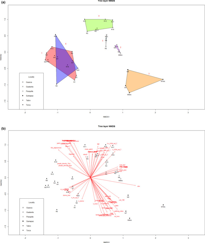
NMDS graphs of the tree layer. (a) Ordination graph of plots in tree species space for axis 1–2: cluster analysis groups are outlined. (b) Ordination graph of plots in tree species space with plotted variables for axis 1–2, with only the variables with ‘p.max = 0.05’ plotted.

The variables that most correlated with the ordination axes (R _Sq > 0.35 for any of the 3 ordination axis, Table 1) and therefore with species composition and abundances are depicted clockwise. For full variable names and acronyms please refer to Appendix A2

.

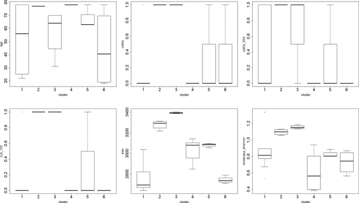
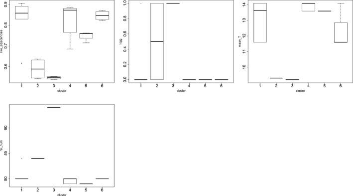
Boxplot of analysis of variance for tree layer groups variables. Only variables that significantly differed among various tree groups (Figure 2) are shown. From right to left: age; presence of cattle inside the plot; (c) presence of cattle within 50 m from the plot; presence of cultivated fields within 100 m from the plot; elevation; Shannon's landscape diversity in 1 km buffer; Like adjacencies in 1 km buffer; logging; mean annual temperature; relative humidity.

APPENDIX A7.

NMDS variables correlation with ordination axes for tree and understory layer

TREES

Variable	NMDS1	NMDS2	R sq	p
elev	0.986936	−0.16111	0.842327	.001
rel_hum	0.557264	−0.83034	0.814799	.001
like_adjacencies	−0.77575	0.631046	0.715877	.001
splitting_index	0.647679	−0.76191	0.712051	.001
patch_cohesion_index	−0.61603	0.787721	0.681776	.001
logg	0.516505	−0.85628	0.633668	.001
greatest_patch	−0.54231	0.84018	0.62502	.001
largest_patch_index	−0.54197	0.840398	0.624739	.001
land_cover	−0.53243	0.846474	0.612971	.001
landscape_porportion	−0.53186	0.846834	0.612778	.001
overall_core	−0.64958	0.760295	0.590216	.001
mean_T	−0.5827	0.812684	0.538388	.001
landscape_shannon	0.392306	−0.91983	0.53266	.001
effective_meshsize	−0.47047	0.882414	0.519565	.002
landscape_division	0.470396	−0.88246	0.519501	.002
%n_CON_ind_T	0.598542	0.801091	0.498647	.001
cult_100	0.828407	−0.56013	0.489726	.001
cattle	0.69714	−0.71693	0.487354	.001
n_CON_ind_T	0.728414	0.685137	0.474397	.001
landscape_simpson	0.333984	−0.94258	0.450877	.003
mliqC	0.917959	0.396676	0.430102	.001
cattle_100	0.535527	−0.84452	0.421884	.003
age	0.230218	0.973139	0.407116	.004
cattle_50m	0.706548	−0.70766	0.387378	.006
road_dist	0.908312	0.418293	0.359839	.001
landscape_pielou	0.549647	−0.8354	0.353878	.004
edge_density	0.922612	0.385729	0.343423	.002
n_patches	0.715658	−0.69845	0.343347	.004
patch_density	0.716517	−0.69757	0.342699	.004
edge_lenght	0.922698	0.385524	0.341936	.002
m_DBH	0.523014	0.852324	0.316577	.004
n.10DBH	0.360665	0.932695	0.29713	.007
fragment	−0.68563	0.727951	0.263566	.016
stems_tree	−0.84893	−0.5285	0.261082	.014
edge	0.690298	−0.72352	0.256775	.025
%n_CON_sp_T	0.596982	0.802255	0.254204	.013
people_density_1km	−0.91227	0.409586	0.253024	.015
mmoss	0.908742	0.417359	0.245418	.022
mean_prec	0.925366	0.379075	0.245257	.013
mean_H	0.356376	0.934343	0.223591	.017
m_cov_inv_U	−0.95141	−0.30794	0.217533	.025
nn_distance	0.589863	−0.8075	0.216971	.031
people_density_5km	−0.92481	0.380421	0.209615	.032
n_inv_sp_U	−0.6223	−0.78278	0.20597	.027
Giniwe	−0.92763	−0.37349	0.20516	.032
mcobT	0.216899	0.976194	0.204958	.028
TPD	−0.78427	−0.62042	0.201613	.044
X._all	0.468041	−0.88371	0.200479	.041
path_dist	0.685608	−0.72797	0.195792	.048
protected	0.615398	0.788216	0.195422	.04
mean_patch	−0.06022	0.998185	0.194229	.042
Giniun	−0.92716	−0.37466	0.185068	.051
HsesMPD	0.988703	−0.14989	0.176882	.068
HsesMNTD	0.348156	−0.93744	0.171425	.065
n_CON_sp_T	0.648282	0.761401	0.17061	.067
cult_50m	0.96786	0.25149	0.16273	.074
n_stems	−0.45592	−0.89002	0.160024	.075
TsesMNTD	−0.81931	−0.57335	0.159924	.081
smallest_patch	0.118311	0.992977	0.156713	.07
median_patch	0.117137	0.993116	0.155408	.075
n_trees	0.219077	−0.97571	0.154968	.096
AGBplot	0.998705	−0.05088	0.154366	.095
cult_500	0.507842	−0.86145	0.153806	.098
mleaf	−0.85047	−0.52603	0.152094	.095
HPD	−0.228	−0.97366	0.150516	.095
TsesPD	−0.51544	−0.85693	0.148752	.102
morqT	0.372927	0.927861	0.145118	.083
mbrioT	−0.13913	0.990274	0.144544	.099
mhelC	−0.99549	0.09491	0.14296	.097
n_FST_ind_T	0.034581	−0.9994	0.141519	.125
H_var	0.642211	0.766528	0.141257	.12
FD	−0.96828	−0.24987	0.140421	.116
mCWD	0.756802	−0.65364	0.137304	.115
FRic	−0.19979	−0.97984	0.137234	.117
HMPD	0.97027	−0.24202	0.129168	.143
TsesMPD	0.417913	−0.90849	0.127914	.142
other	−0.97008	−0.2428	0.126107	.117
mliqT	0.995431	0.095486	0.124934	.171
HsesPD	0.176577	−0.98429	0.121806	.148
mbroT	0.145699	0.989329	0.121332	.176
TsesMNTDABU	−0.99881	0.048778	0.119051	.149
mbroC	−0.26677	0.96376	0.116187	.166
mhelT	−0.16551	0.986208	0.115102	.146
TSR	−0.92753	−0.37375	0.113505	.181
fractal_dimesion_index	0.501947	0.864899	0.110553	.182
m_patchshape_ratio	−0.13742	−0.99051	0.103988	.201
mAGBT	0.649443	0.760411	0.103937	.215
n_sp.10DBH	−0.80905	−0.58774	0.101004	.225
TMPD	0.336675	−0.94162	0.098842	.225
mcobC	0.265827	0.964021	0.097694	.216
sol_rad	−0.17591	0.984406	0.095741	.241
north	−0.40907	−0.9125	0.093814	.22
TPIELOU	0.314002	−0.94942	0.093106	.219
RaoQ	0.764773	−0.6443	0.092153	.264
house_dist	0.316094	0.948728	0.085966	.272
slope	−0.89386	0.448348	0.085597	.29
Hshann	0.169443	−0.98554	0.083351	.282
cattle_500	0.292148	−0.95637	0.080359	.306
n_sp.20DBH	−0.76282	0.646616	0.077075	.32
HSR	−0.34487	−0.93865	0.075683	.323
TMNTD	−0.84452	−0.53553	0.07518	.339
TMPDABU	0.162029	−0.98679	0.074487	.329
Tsimp	0.02132	−0.99977	0.074268	.306
HMNTD	0.7732	−0.63416	0.073592	.32
msoil	−0.6291	0.777325	0.071115	.372
TMNTDABU	−0.99015	−0.14002	0.06572	.38
%_5	−0.20588	−0.97858	0.06549	.365
HsesMNTDABU	−0.52315	−0.85224	0.064366	.377
n.20DBH	0.16129	0.986907	0.060851	.392
Tshann	−0.17924	−0.9838	0.060737	.393
n_FST_sp_T	−0.25137	−0.96789	0.058602	.413
mundstr	−0.55902	−0.82915	0.056845	.435
HPIELOU	0.440781	−0.89761	0.056559	.413
FEve	0.222091	0.975026	0.052515	.481
east	−0.59224	−0.80576	0.051569	.482
Hsimp	0.302214	−0.95324	0.049729	.482
FDis	0.420161	−0.90745	0.046219	.516
DBH_var	0.953164	0.302455	0.043325	.537
n_inv_sp_T	−0.17768	0.984088	0.038882	.571
HsesMPDABU	0.262408	0.964957	0.038792	.567
max_H	0.943325	0.33187	0.038476	.527
track_dist	0.613653	0.789576	0.036408	.575
FDiv	0.063578	−0.99798	0.031273	.634
TsesMPDABU	0.772151	−0.63544	0.029198	.665
morqC	−0.22709	0.973873	0.027614	.666
m_H_understory	0.719951	0.694025	0.018554	.754
HMPDABU	0.997157	0.075357	0.012729	.835
tour	0.074111	0.99725	0.011967	.849
m_cov_nat_U	−0.04515	−0.99898	0.011738	.837
HMNTDABU	−0.99539	−0.09595	0.011378	.848
mbrioC	0.532531	0.84641	0.009829	.886
n_large_trees	−0.57682	0.816872	0.003727	.948

UNDERSTORY

Variable	NMDS1	NMDS2	R sq	p
elev	0.9541	−0.2994	0.7424	.001
%n_CON_ind_T	0.6972	0.7169	0.7030	.001
mliqC	0.8629	−0.5054	0.6210	.001
fragment	−0.4236	0.9058	0.6192	.001
n_CON_ind_T	0.7564	0.6542	0.5868	.001
overall_core	−0.5046	0.8633	0.5779	.001
nn_distance	0.2311	−0.9729	0.5678	.001
n_CON_sp_T	0.4123	0.9110	0.5652	.001
%n_CON_sp_T	0.4612	0.8873	0.5638	.001
road_dist	0.8779	−0.4788	0.5522	.001
edge_density	0.7744	−0.6327	0.5467	.001
edge_lenght	0.7760	−0.6307	0.5458	.001
m_DBH	0.5210	0.8536	0.5361	.001
like_adjacencies	−0.7263	0.6873	0.5287	.001
landscape_pielou	0.3249	−0.9457	0.5282	.001
people_density_1km	−0.6546	0.7560	0.4927	.001
landscape_simpson	0.1586	−0.9873	0.4885	.001
mAGBT	0.5001	0.8659	0.4860	.001
people_density_5km	−0.6587	0.7524	0.4508	.001
effective_meshsize	−0.3264	0.9452	0.4345	.001
landscape_division	0.3269	−0.9450	0.4341	.001
landscape_shannon	0.2587	−0.9660	0.4300	.001
n_stems	−0.3517	−0.9361	0.4254	.001
land_cover	−0.4475	0.8943	0.4112	.002
landscape_porportion	−0.4483	0.8939	0.4105	.002
n_trees	−0.0938	−0.9956	0.4001	.001
cult_500	0.2316	−0.9728	0.3953	.001
mean_H	0.6510	0.7591	0.3926	.001
n.20DBH	0.3331	0.9429	0.3919	.001
greatest_patch	−0.4765	0.8792	0.3789	.003
largest_patch_index	−0.4773	0.8787	0.3783	.003
H_var	0.7528	0.6583	0.3781	.002
mean_patch	0.1234	0.9924	0.3757	.001
age	0.5183	0.8552	0.3631	.001
cattle_100	0.4406	−0.8977	0.3629	.002
n.10DBH	0.5471	0.8371	0.3616	.002
DBH_var	0.3904	0.9206	0.3529	.001
n_patches	0.5521	−0.8338	0.3414	.002
m_patchshape_ratio	−0.2250	−0.9744	0.3411	.001
patch_density	0.5518	−0.8340	0.3409	.002
TsesMNTD	−0.6189	0.7855	0.3379	.004
fractal_dimesion_index	0.3886	0.9214	0.3230	.001
AGBplot	0.6484	0.7613	0.3213	.002
stems_tree	−0.5974	−0.8020	0.3089	.006
mbroT	0.3658	0.9307	0.3069	.005
TsesMNTDABU	−0.4415	0.8973	0.3031	.009
mbroC	0.1503	0.9886	0.3008	.007
median_patch	0.2472	0.9690	0.2962	.002
smallest_patch	0.2492	0.9685	0.2959	.003
TMNTDABU	−0.3654	0.9309	0.2951	.007
n_sp.20DBH	−0.2002	0.9798	0.2940	.003
mmoss	0.7328	−0.6804	0.2935	.011
protected	0.9616	−0.2746	0.2768	.005
mcobT	0.5901	0.8073	0.2766	.009
cattle_50m	0.6646	−0.7472	0.2739	.01
cattle	0.6734	−0.7392	0.2683	.013
HMPD	0.4505	0.8928	0.2675	.013
n_FST_ind_T	−0.0733	−0.9973	0.2597	.017
TsesPD	−0.5789	0.8154	0.2562	.015
HsesMPD	0.5830	0.8125	0.2534	.016
TMPD	0.0440	0.9990	0.2481	.02
morqT	0.7128	0.7014	0.2452	.019
TMNTD	−0.5690	0.8223	0.2441	.017
patch_cohesion_index	−0.7432	0.6691	0.2368	.017
n_large_trees	0.1904	0.9817	0.2271	.019
mleaf	−0.9005	−0.4348	0.2246	.025
mcobC	0.6767	0.7362	0.2211	.031
mliqT	0.7831	−0.6219	0.2199	.026
sol_rad	0.3578	−0.9338	0.2166	.029
tour	0.2983	−0.9545	0.2130	.037
edge	0.6123	−0.7907	0.2109	.033
splitting_index	0.8714	−0.4905	0.2087	.028
cult_100	0.8494	−0.5278	0.2079	.034
n_inv_sp_U	−0.7628	−0.6466	0.2069	.034
TsesMPD	0.0840	0.9965	0.2059	.037
mhelT	0.2106	0.9776	0.1995	.038
max_H	0.7056	0.7086	0.1992	.043
mean_prec	0.8755	−0.4832	0.1907	.053
house_dist	0.5493	−0.8356	0.1902	.055
TMPDABU	0.1551	0.9879	0.1872	.049
TsesMPDABU	0.1618	0.9868	0.1862	.046
Giniwe	−0.5636	−0.8260	0.1815	.049
n_sp.10DBH	−0.6307	0.7761	0.1762	.061
mhelC	−0.4689	0.8833	0.1745	.06
TPD	−0.6826	0.7308	0.1737	.083
cattle_500	0.0966	−0.9953	0.1703	.068
morqC	0.3163	0.9487	0.1693	.069
mean_T	−0.8561	0.5168	0.1561	.075
msoil	−0.2462	0.9692	0.1506	.102
Giniun	−0.5473	−0.8369	0.1506	.096
other	−0.9893	0.1462	0.1492	.078
mundstr	−0.4332	0.9013	0.1469	.108
HMNTD	0.1854	−0.9827	0.1441	.117
m_cov_inv_U	−0.9990	0.0445	0.1427	.124
FDiv	−0.1388	0.9903	0.1402	.122
%_all	0.3145	−0.9492	0.1391	.124
cult_50m	0.7689	−0.6394	0.1348	.101
HsesMNTDABU	−0.8341	−0.5516	0.1219	.157
HPIELOU	0.1081	−0.9941	0.1217	.143
rel_hum	0.8988	−0.4384	0.1211	.152
logg	0.6668	−0.7452	0.1135	.157
m_cov_nat_U	−0.1436	0.9896	0.1131	.167
mCWD	0.6105	0.7920	0.1075	.171
%_5	−0.3215	−0.9469	0.1066	.196
east	−0.8527	−0.5223	0.1063	.162
HsesMNTD	−0.0559	−0.9984	0.1007	.216
HsesMPDABU	0.0924	0.9957	0.0993	.197
TPIELOU	0.4560	0.8900	0.0941	.242
n_FST_sp_T	−0.2760	−0.9611	0.0928	.267
RaoQ	0.8038	0.5949	0.0841	.288
slope	−0.9069	−0.4214	0.0770	.335
FD	−0.7789	0.6272	0.0705	.365
Tshann	0.0868	0.9962	0.0681	.372
Tsimp	0.2034	0.9791	0.0680	.385
track_dist	0.9412	0.3377	0.0674	.375
HPD	−0.8959	0.4443	0.0578	.428
HMNTDABU	−0.7611	−0.6487	0.0570	.42
Hshann	−0.1013	−0.9949	0.0562	.434
FEve	0.4481	0.8940	0.0544	.433
TSR	−0.7679	0.6406	0.0532	.46
mbrioT	0.0471	0.9989	0.0521	.44
m_H_understory	0.2972	0.9548	0.0512	.47
FDis	0.4714	0.8819	0.0497	.486
path_dist	0.7276	0.6860	0.0390	.572
Hsimp	0.0455	−0.9990	0.0381	.57
n_inv_sp_T	0.2033	−0.9791	0.0380	.575
HSR	−0.7537	0.6573	0.0378	.568
north	−0.7210	−0.6929	0.0376	.566
FRic	−0.7253	0.6885	0.0244	.722
HsesPD	−0.4330	−0.9014	0.0243	.722
mbrioC	0.7545	0.6563	0.0112	.868
HMPDABU	0.3434	0.9392	0.0067	.91

APPENDIX A8.

NMDS understory layer graphs and analysis of variance boxplots

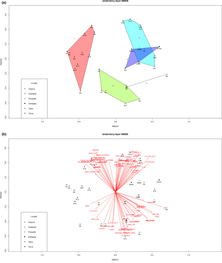
NMDS of understory. (a) ordination graph of plots in understory species space for axis 1–2: no group could be visually distinguished and cluster analysis groups are outlined (b) Ordination graph of plots in understory species space with plotted variables for axis 1–2, with only the variables with ‘p.max = 0.05’ plotted. A table offering variable correlations with the ordination axes is available in Appendix A8.

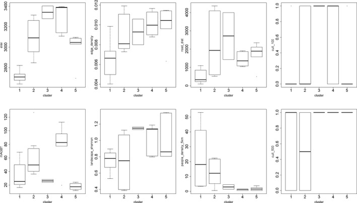
Boxplot of analysis of variance for understory groups variables. Only variables that significantly differed among various understory groups are shown: elevation; edge density in 1 km buffer; distances from roads; presence of cultivated fields within 100 m from the plot; mean tree AGB; Shannon's landscape diversity in 1 km buffer; people population density in 5 km buffer; presence of cultivated fields within 500 m from the plot.

Calbi M, Fajardo‐Gutiérrez F, Posada JM, Lücking R, Brokamp G, Borsch T. Seeing the wood despite the trees: Exploring human disturbance impact on plant diversity, community structure, and standing biomass in fragmented high Andean forests. Ecol Evol. 2021;11:2110–2172. 10.1002/ece3.7182

DATA AVAILABILITY STATEMENT

The tree layer and understory sampling datasets and the complete table of variables have been submitted to the Dryad digital repository (https://doi.org/10.5061/dryad.z612jm6b5).

REFERENCES

- Acuña, C. A. (2013). Potencial de regeneración de rastrojos y bosques secundarios en la sabana de Bogotá. Master’s degree Thesis. Pontificia Universidad Javeriana. [Google Scholar]
- Aldana, A. M. , Villanueva, B. , Cano, Á. , Correa, D. F. , Umaña, M. N. , Casas, L. F. , Cárdenas, S. , Henao‐Diaz, L. F. , & Stevenson, P. R. (2017). Drivers of biomass stocks in Northwestern South American forests: Contributing new information on the Neotropics. Forest Ecology and Management, 389, 86–95. 10.1016/j.foreco.2016.12.023 [DOI] [Google Scholar]
- Álvarez‐Dávila, E. , Cayuela, L. , González‐Caro, S. , Aldana, A. M. , Stevenson, P. R. , Phillips, O. , Cogollo, Á. , Peñuela, M. C. , von Hildebrand, P. , Jiménez, E. , Melo, O. , Londoño‐Vega, A. C. , Mendoza, I. , Velásquez, O. , Fernández, F. , Serna, M. , Velázquez‐Rua, C. , Benítez, D. , & Rey‐Benayas, J. M. (2017). Forest biomass density across large climate gradients in northern South America is related to water availability but not with temperature. PLoS One, 12(3), e0171072. 10.1371/journal.pone.0171072 [DOI] [PMC free article] [PubMed] [Google Scholar]
- Ampoorter, E. , Baeten, L. , Koricheva, J. , Vanhellemont, M. , & Verheyen, K. (2014). Do diverse overstoreys induce diverse understoreys? Lessons learnt from an experimental–observational platform in Finland. Forest Ecology and Management, 318, 206–215. 10.1016/j.foreco.2014.01.030 [DOI] [Google Scholar]
- Anselm, N. , Brokamp, G. , & Schütt, B. (2018). Assessment of land cover change in peri‐urban high andean environments South of Bogotá, Colombia. Land, 7(2), 75. 10.3390/land7020075 [DOI] [Google Scholar]
- Anselm, N. , Rojas, O. , Brokamp, G. , & Schütt, B. (2020). Spatiotemporal variability of precipitation and its statistical relations to ENSO in the high Andean Rio Bogotá watershed, Colombia. Earth Interactions, 24(3), 1–17. 10.1175/EI-D-19-0019.1 [DOI] [Google Scholar]
- Armenteras, D. , Gast, F. , & Villareal, H. (2003). Andean forest fragmentation and the representativeness of protected natural areas in the eastern Andes, Colombia. Biological Conservation, 113(2), 245–256. 10.1016/S0006-3207(02)00359-2 [DOI] [Google Scholar]
- Avella, A. , Torres, S. , Gómez, W. , & Pardo, M. (2014). Los páramos y bosques altoandinos del pantano de Monquentiva o pantano de Martos (Guatavita, Cundinamarca, Colombia): Caracterización ecológica y estado de conservación. Biota Colombiana, 15(1), 3–39. [Google Scholar]
- Bach, K. , Kessler, M. , & Gradstein, S. (2007). A simulation approach to determine statistical significance of species turnover peaks in a species‐rich tropical cloud forest. Diversity and Distributions, 13(6), 863–870. 10.1111/j.1472-4642.2007.00357.x [DOI] [Google Scholar]
- Batke, S. P. , Murphy, B. R. , Hill, N. , & Kelly, D. L. (2015). Can air humidity and temperature regimes within cloud forest canopies be predicted from bryophyte and lichen cover? Ecological Indicators, 56, 1–5. 10.1016/j.ecolind.2015.03.022 [DOI] [Google Scholar]
- Battles, J. J. , Shlisky, A. J. , Barrett, R. H. , Heald, R. C. , & Allen‐Diaz, B. H. (2001). The effects of forest management on plant species diversity in a Sierran conifer forest. Forest Ecology and Management, 146(1–3), 211–222. 10.1016/S0378-1127(00)00463-1 [DOI] [Google Scholar]
- Berenguer, E. , Ferreira, J. , Gardner, T. A. , Aragão, L. E. O. C. , De Camargo, P. B. , Cerri, C. E. , Durigan, M. , Oliveira, R. C. D. , Vieira, I. C. G. , & Barlow, J. (2014). A large‐scale field assessment of carbon stocks in human‐modified tropical forests. Global Change Biology, 20(12), 3713–3726. 10.1111/gcb.12627 [DOI] [PubMed] [Google Scholar]
- Bourdier, T. , Cordonnier, T. , Kunstler, G. , Piedallu, C. , Lagarrigues, G. , & Courbaud, B. (2016). Tree size inequality reduces forest productivity: An analysis combining inventory data for ten European species and a light competition model. PLoS One, 11(3), e0151852. 10.1371/journal.pone.0151852 [DOI] [PMC free article] [PubMed] [Google Scholar]
- Bovendorp, R. S. , Brum, F. T. , McCleery, R. A. , Baiser, B. , Loyola, R. , Cianciaruso, M. V. , & Galetti, M. (2019). Defaunation and fragmentation erode small mammal diversity dimensions in tropical forests. Ecography, 42(1), 23–35. 10.1111/ecog.03504 [DOI] [Google Scholar]
- Brown, A. D. , & Kappelle, M. (2001). Introducción a los bosques nublados del neotrópico: Una síntesis regional (pp. 25–40). Bosques Nublados del Neotrópico Editorial INBio. [Google Scholar]
- Buuren S. V., Groothuis‐Oudshoorn K. (2011). mice: Multivariate Imputation by Chained Equations in R. Journal of Statistical Software, 45(3), 1–67. 10.18637/jss.v045.i03 [DOI] [Google Scholar]
- Cabrera, O. , Benítez, Á. , Cumbicus, N. , Naranjo, C. , Ramón, P. , Tinitana, F. , & Escudero, A. (2019). Geomorphology and altitude effects on the diversity and structure of the vanishing montane forest of southern ecuador. Diversity, 11(3), 32. 10.3390/d11030032 [DOI] [Google Scholar]
- Calbi, M. , Clerici, N. , Borsch, T. , & Brokamp, G. (2020). Reconstructing long term high Andean forest dynamics using historical aerial imagery: A case study in Colombia. Forests, 11(8), 788. 10.3390/f11080788 [DOI] [Google Scholar]
- Cantillo Higuera, E. E. , & Gracia, C. M. (2013). Diversidad y caracterización florística de la vegetación natural en tres sitios de los cerros orientales de Bogotá D. C. Colombia Forestal, 16(2), 228. [Google Scholar]
- Cavelier, J. , Lizcaino, D. , & Pulido, M. (2001). Bosques nublados del neotrópico: Colombia. (p. 700). Bosques nublados del neotrópico Instituto Nacional de Biodiversidad Santo Domingo de Heredia. [Google Scholar]
- Chaplin‐Kramer, R. , Sharp, R. P. , Mandle, L. , Sim, S. , Johnson, J. , Butnar, I. , Milà i Canals, L. , Eichelberger, B. A. , Ramler, I. , Mueller, C. , McLachlan, N. , Yousefi, A. , King, H. , & Kareiva, P. M. (2015). Spatial patterns of agricultural expansion determine impacts on biodiversity and carbon storage. Proceedings of the National Academy of Sciences, 112(24), 7402–7407. 10.1073/pnas.1406485112 [DOI] [PMC free article] [PubMed] [Google Scholar]
- Chave, J. , Coomes, D. , Jansen, S. , Lewis, S. L. , Swenson, N. G. , & Zanne, A. E. (2009). Towards a worldwide wood economics spectrum. Ecology Letters, 12(4), 351–366. 10.1111/j.1461-0248.2009.01285.x [DOI] [PubMed] [Google Scholar]
- Chave, J. , Réjou‐Méchain, M. , Búrquez, A. , Chidumayo, E. , Colgan, M. S. , Delitti, W. B. C. , Duque, A. , Eid, T. , Fearnside, P. M. , Goodman, R. C. , Henry, M. , Martínez‐Yrízar, A. , Mugasha, W. A. , Muller‐Landau, H. C. , Mencuccini, M. , Nelson, B. W. , Ngomanda, A. , Nogueira, E. M. , Ortiz‐Malavassi, E. , … Vieilledent, G. (2014). Improved allometric models to estimate the aboveground biomass of tropical trees. Global Change Biology, 20(10), 3177–3190. 10.1111/gcb.12629 [DOI] [PubMed] [Google Scholar]
- Chaves, M. E. , & Arango, N. (1998). Informe nacional sobre el estado de la biodiversidad: Diversidad biológica: Instituto de Investigación de Recursos Biológicos. Alexander von Humboldt. [Google Scholar]
- Chun, J.‐H. , & Lee, C.‐B. (2018). Partitioning the regional and local drivers of phylogenetic and functional diversity along temperate elevational gradients on an East Asian peninsula. Scientific Reports, 8(1), 2853. 10.1038/s41598-018-21266-4 [DOI] [PMC free article] [PubMed] [Google Scholar]
- Cleef, A. M. (1981). The vegetation of the páramos of the Colombian Cordillera Oriental. Mededelingen Van Het Botanisch Museum En Herbarium Van De Rijksuniversiteit Te Utrecht, 481(1), 1–320. [Google Scholar]
- Congedo, L. (2016). Semi‐automatic classification plugin documentation. Release. 4(0.1), 29. [Google Scholar]
- Cortés, S. (2008). La vegetación boscosa y arbustiva de la cuenca alta del río Bogotá/Forest and shrub vegetation of the upper basin of the Bogotá river. van der Hammen T. Rangel‐Churio O. & Cleef A. (Eds.), La cordillera Oriental colombiana, transecto Sumapaz. Estudios de Ecosistemas Tropandinos, 7, (915–960). Berlin‐Stuttgart: J. Cramer. [Google Scholar]
- Cortés, S. , Van der Hammen, T. , & Rangel, O. (1999). Comunidades vegetales y patrones de degradación y sucesión en la vegatación de los cerros occidentales de Chia Cundinamarca‐Colombia. Revista De La Academia Colombiana Deficiencias, 23(89), 529–554. [Google Scholar]
- Cuatrecasas, J. (1934). Observaciones geobotánicas en Colombia. Junta para Ampliación de Estudios e Investigaciones Científicas. [Google Scholar]
- Cuatrecasas, J. (1958). Aspectos de la vegetación natural de Colombia. Revista De La Academia Colombiana De Ciencias Exactas, Físicas Y Naturales., 10(40), 221–268. [Google Scholar]
- DANE Departamento Administrativo Nacional de Estadística (DANE) , (2018). Retrieved from http://www.dane.gov.co/?descarga‐marco‐geoestadistico‐nacional
- DANE Departamento Administrativo Nacional de Estadística (DANE) (2019). Retrieved from https://geoportal.dane.gov.co/?estimaciones‐proyecciones
- D'Angelo, S. A. , Andrade, A. C. , Laurance, S. G. , Laurance, W. F. , & Mesquita, R. C. (2004). Inferred causes of tree mortality in fragmented and intact Amazonian forests. Journal of Tropical Ecology, 20(2), 243–246. [Google Scholar]
- de Paula, M. D. , Costa, C. P. A. , & Tabarelli, M. (2011). Carbon storage in a fragmented landscape of Atlantic forest: The role played by edge‐affected habitats and emergent trees. Tropical Conservation Science, 4(3), 349–358. 10.1177/194008291100400310 [DOI] [Google Scholar]
- Diaz, S. , & Cabido, M. (2001). Vive la difference: Plant functional diversity matters to ecosystem processes. Trends in Ecology & Evolution, 16(11), 646–655. [Google Scholar]
- Ding, Y. , Zang, R. , Letcher, S. G. , Liu, S. , & He, F. (2012). Disturbance regime changes the trait distribution, phylogenetic structure and community assembly of tropical rain forests. Oikos, 121(8), 1263–1270. 10.1111/j.1600-0706.2011.19992.x [DOI] [Google Scholar]
- Etter, A. , McAlpine, C. , & Possingham, H. (2008). Historical patterns and drivers of landscape change in Colombia since 1500: A regionalized spatial approach. Annals of the Association of American Geographers, 98(1), 2–23. 10.1080/00045600701733911 [DOI] [Google Scholar]
- Etter, A. , & van Wyngaarden, W. (2000). Patterns of landscape transformation in Colombia, with emphasis in the Andean region. AMBIO: A Journal of the Human Environment, 29(7), 432–440. 10.1579/0044-7447-29.7.432 [DOI] [Google Scholar]
- Evy, A. , Federico, S. , Harald, A. , Lander, B. , Sigrid, B. , Elisa, C. , Andrea, C. , Mariangela, F. , Kalliopi, R. , Nurlaila, S. N. , Margot, V. , & Kris, V. (2016). Driving mechanisms of overstorey–understorey diversity relationships in European forests. Perspectives in Plant Ecology, Evolution and Systematics, 19, 21–29. 10.1016/j.ppees.2016.02.001 [DOI] [Google Scholar]
- Fahey, R. T. , & Puettmann, K. J. (2007). Ground‐layer disturbance and initial conditions influence gap partitioning of understorey vegetation. Journal of Ecology, 95(5), 1098–1109. 10.1111/j.1365-2745.2007.01283.x [DOI] [Google Scholar]
- Fahrig, L. (2003). Effects of habitat fragmentation on biodiversity. Annual Review of Ecology, Evolution, and Systematics, 34(1), 487–515. 10.1146/annurev.ecolsys.34.011802.132419 [DOI] [Google Scholar]
- Flynn, D. F. , Mirotchnick, N. , Jain, M. , Palmer, M. I. , & Naeem, S. (2011). Functional and phylogenetic diversity as predictors of biodiversity–ecosystem‐function relationships. Ecology, 92(8), 1573–1581. 10.1890/10-1245.1 [DOI] [PubMed] [Google Scholar]
- Forman, R. T. , & Alexander, L. E. (1998). Roads and their major ecological effects. Annual Review of Ecology and Systematics, 29(1), 207–231. 10.1146/annurev.ecolsys.29.1.207 [DOI] [Google Scholar]
- Franco, M. , Betancur, J. , & Franco, P. (2010). Diversidad florística y estructura de remanentes de bosque andino en la zona de amortiguación del Parque Nacional Natural los Nevados, Cordillera Central Colombiana. Caldasia, 32(1), 39–63. [Google Scholar]
- Frenzke, L. , Lederer, A. , Malanin, M. , Eichhorn, K.‐J. , Neinhuis, C. , & Voigt, D. (2016). Plant pressure sensitive adhesives: Similar chemical properties in distantly related plant lineages. Planta, 244(1), 145–154. 10.1007/s00425-016-2496-4 [DOI] [PubMed] [Google Scholar]
- Gentry, A. , & Ortiz, R. (1993). Patrones de composición florística en la Amazonía peruana (pp. 155–166). vegetación húmeda tropical en el llano subandino. [Google Scholar]
- Gentry, A. H. , & Vasquez, R. (1993). A field guide to the families and genera of woody plants of northwest South America (Colombia, Ecuador, Peru): with supplementary notes on herbaceous taxa. [Google Scholar]
- Gerhold, P. , Cahill, J. F. , Winter, M. , Bartish, I. V. , & Prinzing, A. (2015). Phylogenetic patterns are not proxies of community assembly mechanisms (they are far better). Functional Ecology, 29(5), 600–614. 10.1111/1365-2435.12425 [DOI] [Google Scholar]
- Girardin, C. A. J. , Espejob, J. E. S. , Doughty, C. E. , Huasco, W. H. , Metcalfe, D. B. , Durand‐Baca, L. , Marthews, T. R. , Aragao, L. E. O. C. , Farfán‐Rios, W. , García‐Cabrera, K. , Halladay, K. , Fisher, J. B. , Galiano‐Cabrera, D. F. , Huaraca‐Quispe, L. P. , Alzamora‐Taype, I. , Eguiluz‐Mora, L. , ‐Revilla, N. S. , Silman, M. R. , Meir, P. , & Malhi, Y. (2014). Productivity and carbon allocation in a tropical montane cloud forest in the Peruvian Andes. Plant Ecology & Diversity, 7(1–2), 107–123. 10.1080/17550874.2013.820222 [DOI] [Google Scholar]
- González, W. , Llambí, L. D. , Smith, J. K. , & Gámez, L. E. (2011). Dinámica sucesional del componente arbóreo en la zona de transición bosque‐Páramo en Los Andes Tropicales. Ecotrópicos, 24(1), 60–79. [Google Scholar]
- Halpern, C. B. , & Lutz, J. A. (2013). Canopy closure exerts weak controls on understory dynamics: A 30‐year study of overstory–understory interactions. Ecological Monographs, 83(2), 221–237. 10.1890/12-1696.1 [DOI] [Google Scholar]
- Halpern, C. B. , & Spies, T. A. (1995). Plant species diversity in natural and managed forests of the Pacific Northwest. Ecological Applications., 5(4), 913–934. 10.2307/2269343 [DOI] [Google Scholar]
- Handcock, M. S. (2016). Relative Distribution Methods. Version 1.6–6. R package. [Google Scholar]
- Heath, J. , & Binswanger, H. (1996). Natural resource degradation effects of poverty and population growth are largely policy‐induced: The case of Colombia. Environment and Development Economics, 1(1), 65–84. 10.1017/S1355770X00000383 [DOI] [Google Scholar]
- Hertzog, L. R. , Boonyarittichaikij, R. , Dekeukeleire, D. , de Groote, S. R. E. , van Schrojenstein Lantman, I. M. , Sercu, B. K. , Smith, H. K. , de la Peña, E. , Vandegehuchte, M. L. , Bonte, D. , Martel, A. , Verheyen, K. , Lens, L. , & Baeten, L. (2019). Forest fragmentation modulates effects of tree species richness and composition on ecosystem multifunctionality. Ecology, 100(4), e02653. [DOI] [PubMed] [Google Scholar]
- Hill, J. , & Curran, P. (2001). Species composition in fragmented forests: Conservation implications of changing forest area. Applied Geography, 21(2), 157–174. 10.1016/S0143-6228(01)00002-9 [DOI] [Google Scholar]
- Homeier, J. , Breckle, S. W. , Günter, S. , Rollenbeck, R. T. , & Leuschner, C. (2010). Tree diversity, forest structure and productivity along altitudinal and topographical gradients in a species‐rich Ecuadorian montane rain forest. Biotropica, 42(2), 140–148. 10.1111/j.1744-7429.2009.00547.x [DOI] [Google Scholar]
- Huebner, C. D. , Randolph, J. C. , & Parker, G. R. (1995). Environmental factors affecting understory diversity in second‐growth deciduous forests. American Midland Naturalist, 134, 155–165. 10.2307/2426492 [DOI] [Google Scholar]
- Hurtado‐M A. B., Echeverry‐Galvis M. Á., Salgado‐Negret B., Muñoz J. C., Posada J. M., Norden N. (2020). Little trace of floristic homogenization in peri‐urban Andean secondary forests despite high anthropogenic transformation. Journal of Ecology. 10.1111/1365-2745.13570 [DOI] [Google Scholar]
- IDEAM (2007). Estudio de la Caracterización Climática de Bogotá y Cuenca Alta del Río Tunjuelo. [Google Scholar]
- IDEAM (2015). Atlas Climatológico de Colombia – Interactivo – año 2015. [Google Scholar]
- IGAC (1985). Estudio General de Suelos de los Sectores Sur y Suroeste del Departamento de Cundinamarca (Vol. 1). IGAC. 978‐958‐8067‐73‐5. [Google Scholar]
- Jung, M. (2013). LecoS‐A QGIS plugin for automated landscape ecology analysis. PeerJ PrePrints. Report No.: 2167–9843. [Google Scholar]
- Keith, H. , Mackey, B. G. , & Lindenmayer, D. B. (2009). Re‐evaluation of forest biomass carbon stocks and lessons from the world's most carbon‐dense forests. Proceedings of the National Academy of Sciences, 106(28), 11635–11640. 10.1073/pnas.0901970106 [DOI] [PMC free article] [PubMed] [Google Scholar]
- Kembel, S. W. , Cowan, P. D. , Helmus, M. R. , Cornwell, W. K. , Morlon, H. , Ackerly, D. D. , Blomberg, S. P. , & Webb, C. O. (2010). Picante: R tools for integrating phylogenies and ecology. Bioinformatics, 26(11), 1463–1464. 10.1093/bioinformatics/btq166 [DOI] [PubMed] [Google Scholar]
- Killeen, T. J. , Douglas, M. , Consiglio, T. , Jørgensen, P. M. , & Mejia, J. (2007). Dry spots and wet spots in the Andean hotspot. Journal of Biogeography, 34(8), 1357–1373. 10.1111/j.1365-2699.2006.01682.x [DOI] [Google Scholar]
- Köster, N. , Friedrich, K. , Nieder, J. , & Barthlott, W. (2009). Conservation of epiphyte diversity in an Andean landscape transformed by human land use. Conservation Biology, 23(4), 911–919. 10.1111/j.1523-1739.2008.01164.x [DOI] [PubMed] [Google Scholar]
- Krömer, T. , Kessler, M. , & Gradstein, S. R. (2007). Vertical stratification of vascular epiphytes in submontane and montane forest of the Bolivian Andes: The importance of the understory. Plant Ecology, 189(2), 261–278. 10.1007/s11258-006-9182-8 [DOI] [Google Scholar]
- Kupfer, J. A. , Webbeking, A. L. , & Franklin, S. B. (2004). Forest fragmentation affects early successional patterns on shifting cultivation fields near Indian Church, Belize. Agriculture, Ecosystems & Environment, 103(3), 509–518. 10.1016/j.agee.2003.11.011 [DOI] [Google Scholar]
- Kusuma, Y. W. C. , Rembold, K. , Tjitrosoedirdjo, S. S. , & Kreft, H. (2018). Tropical rainforest conversion and land use intensification reduce understorey plant phylogenetic diversity. Journal of Applied Ecology, 55(5), 2216–2226. 10.1111/1365-2664.13201 [DOI] [Google Scholar]
- Laliberté, E. , & Legendre, P. (2010). A distance‐based framework for measuring functional diversity from multiple traits. Ecology, 91(1), 299–305. 10.1890/08-2244.1 [DOI] [PubMed] [Google Scholar]
- Laliberté, E. , Legendre, P. , Shipley, B. , & Laliberté, M. E. (2014). Package ‘FD’. Measuring functional diversity from multiple traits, and other tools for functional ecology. [DOI] [PubMed] [Google Scholar]
- Latham, P. A. , Zuuring, H. R. , & Coble, D. W. (1998). A method for quantifying vertical forest structure. Forest Ecology and Management, 104(1–3), 157–170. 10.1016/S0378-1127(97)00254-5 [DOI] [Google Scholar]
- Laurance, W. F. , & Bierregaard, R. O. (1997). Tropical forest remnants: Ecology, management, and conservation of fragmented communities. University of Chicago Press. [Google Scholar]
- Laurance, W. F. , Delamônica, P. , Laurance, S. G. , Vasconcelos, H. L. , & Lovejoy, T. E. (2000). Conservation: Rainforest fragmentation kills big trees. Nature, 404(6780), 836. 10.1038/35009032 [DOI] [PubMed] [Google Scholar]
- Laurance, W. F. , Nascimento, H. E. M. , Laurance, S. G. , Andrade, A. , Ribeiro, J. E. L. S. , Giraldo, J. P. , Lovejoy, T. E. , Condit, R. , Chave, J. , Harms, K. E. , & D'Angelo, S. (2006). Rapid decay of tree‐community composition in Amazonian forest fragments. Proceedings of the National Academy of Sciences, 103(50), 19010–19014. 10.1073/pnas.0609048103 [DOI] [PMC free article] [PubMed] [Google Scholar]
- Legendre, P. , & Gallagher, E. D. (2001). Ecologically meaningful transformations for ordination of species data. Oecologia, 129(2), 271–280. 10.1007/s004420100716 [DOI] [PubMed] [Google Scholar]
- Letcher, S. G. (2009). Phylogenetic structure of angiosperm communities during tropical forest succession. Proceedings of the Royal Society B: Biological Sciences, 277(1678), 97–104. 10.1098/rspb.2009.0865 [DOI] [PMC free article] [PubMed] [Google Scholar]
- Lexerød, N. L. , & Eid, T. (2006). An evaluation of different diameter diversity indices based on criteria related to forest management planning. Forest Ecology and Management, 222(1–3), 17–28. 10.1016/j.foreco.2005.10.046 [DOI] [Google Scholar]
- Linares, P. V. , & Ríos, O. V. (2004). Dinámica de la dispersión de plantas ornitócoras, reclutamiento y conectividad en fragmentos de bosque altoandino secundario (Reserva Natural Protectora, Cogua Cundinamarca). Acta Biológica Colombiana, 9(2), 121–122. [Google Scholar]
- López, W. , & Duque, Á. (2010). Patrones de diversidad alfa en tres fragmentos de bosques montanos en la región norte de los Andes. Colombia. Revista De Biología Tropical, 58(1), 483–498. [PubMed] [Google Scholar]
- Lumley, T. , & Lumley, M. T. (2013). Package ‘leaps’. Regression Subset Selection. Thomas Lumley Based on Fortran Code by Alan Miller. 2013. Retrieved from http://CRAN.R‐project.org/package=leaps (accessed on 5 September 2020). [Google Scholar]
- Luteyn, J. L. (2002). Diversity, adaptation, and endemism in neotropical Ericaceae: Biogeographical patterns in the Vaccinieae. The Botanical Review, 68(1), 55–87.10.1663/0006‐8101(2002)068[0055:DAAEIN]2.0.CO;2 [Google Scholar]
- Marcantonio, M. , Rocchini, D. , Geri, F. , Bacaro, G. , & Amici, V. (2013). Biodiversity, roads, & landscape fragmentation: Two Mediterranean cases. Applied Geography, 42, 63–72. [Google Scholar]
- Mason, N. W. , Mouillot, D. , Lee, W. G. , & Wilson, J. B. (2005). Functional richness, functional evenness and functional divergence: The primary components of functional diversity. Oikos, 111(1), 112–118. 10.1111/j.0030-1299.2005.13886.x [DOI] [Google Scholar]
- McCune, B. , & Mefford, M. J. (2015). PC‐ORD Version 7.287. Multivariate Analysis of Ecological Data. MjM Software. [Google Scholar]
- Mendoza S., J. E. , & Etter R., A. (2002). Multitemporal analysis (1940–1996) of land cover changes in the southwestern Bogotá highplain (Colombia). Landscape and Urban Planning, 59(3), 147–158. 10.1016/S0169-2046(02)00012-9 [DOI] [Google Scholar]
- Menon, S. , Denman, K. L. , Brasseur, G. , Chidthaisong, A. , Ciais, P. , Cox, P. M. , Dickinson, R. E. , Hauglustaine, D. , Heinze, C. , Holland, E. , & Jacob, D. (2007). Couplings between changes in the climate system and biogeochemistry. Lawrence Berkeley National Lab. (LBNL). [Google Scholar]
- Millspaugh, J. , & Thompson, F. R. (Eds.) (2011). Models for planning wildlife conservation in large landscapes. Academic Press. [Google Scholar]
- Mori, A. S. , Furukawa, T. , & Sasaki, T. (2013). Response diversity determines the resilience of ecosystems to environmental change. Biological Reviews, 88(2), 349–364. 10.1111/brv.12004 [DOI] [PubMed] [Google Scholar]
- Moser, G. , Leuschner, C. , Hertel, D. , Graefe, S. , Soethe, N. , & Iost, S. (2011). Elevation effects on the carbon budget of tropical mountain forests (S Ecuador): The role of the belowground compartment. Global Change Biology, 17, 2211–2226. [Google Scholar]
- Mouchet, M. A. , Villéger, S. , Mason, N. W. , & Mouillot, D. (2010). Functional diversity measures: An overview of their redundancy and their ability to discriminate community assembly rules. Functional Ecology, 24(4), 867–876. 10.1111/j.1365-2435.2010.01695.x [DOI] [Google Scholar]
- Muñoz‐Camacho, J. C. , Hurtado, A. B. , & Norden, N. (2017). Composición florística de tres fragmentos de bosque altoandino en los alrededores de la sabana de Bogotá: Parcelas permanentes del Proyecto Rastrojos. [Google Scholar]
- Munzi, S. , Correia, O. , Silva, P. , Lopes, N. , Freitas, C. , Branquinho, C. , & Pinho, P. (2014). Lichens as ecological indicators in urban areas: Beyond the effects of pollutants. Journal of Applied Ecology, 51(6), 1750–1757. 10.1111/1365-2664.12304 [DOI] [Google Scholar]
- NASA/METI/AIST/Japan Spacesystems, and U.S./Japan ASTER Science Team (2009). ASTER Global Digital Elevation Model [Data set]. NASA EOSDIS Land Processes DAAC. 10.5067/ASTER/ASTGTM.002 [DOI] [Google Scholar]
- Nepstad, D. C. , Moutinho, P. , Dias‐Filho, M. B. , Davidson, E. , Cardinot, G. , Markewitz, D. , Figueiredo, R. , Vianna, N. , Chambers, J. , Ray, D. , & Guerreiros, J. B. (2002). The effects of partial throughfall exclusion on canopy processes, aboveground production, and biogeochemistry of an Amazon forest. Journal of Geophysical Research: Atmospheres, 107(D20), LBA‐53, 10.1029/2001JD000360 [DOI] [Google Scholar]
- Nilsson, M.‐C. , & Wardle, D. A. (2005). Understory vegetation as a forest ecosystem driver: Evidence from the northern Swedish boreal forest. Frontiers in Ecology and the Environment, 3(8), 421–428.10.1890/1540‐9295(2005)003[0421:UVAAFE]2.0.CO;2 [Google Scholar]
- Norden, N. , Letcher, S. G. , Boukili, V. , Swenson, N. G. , & Chazdon, R. (2012). Demographic drivers of successional changes in phylogenetic structure across life‐history stages in plant communities. Ecology, 93(sp8), S70–S82. 10.1890/10-2179.1 [DOI] [Google Scholar]
- Oksanen, J. , Blanchet, F. G. , Kindt, R. , Legendre, P. , Minchin, P. R. , O'hara, R. B. , Simpson, G. L. , Solymos, P. , Stevens, M. H. H. , & Wagner, H. (2013). Community ecology package. R package version, 2–0. [Google Scholar]
- Paine, R. T. , Tegner, M. J. , & Johnson, E. A. (1998). Compounded perturbations yield ecological surprises. Ecosystems, 1(6), 535–545. 10.1007/s100219900049 [DOI] [Google Scholar]
- Parra Sánchez, E. , Armenteras, D. , & Retana, J. (2016). Edge influence on diversity of orchids in Andean cloud forests. Forests, 7(3), 63. 10.3390/f7030063 [DOI] [Google Scholar]
- Parton, W. , Morgan, J. , Smith, D. , Del Grosso, S. , Prihodko, L. , LeCain, D. , Kelly, R. , & Lutz, S. (2012). Impact of precipitation dynamics on net ecosystem productivity. Global Change Biology, 18(3), 915–927. 10.1111/j.1365-2486.2011.02611.x [DOI] [Google Scholar]
- Pérez‐Harguindeguy, N. , Díaz, S. , Garnier, E. , Lavorel, S. , Poorter, H. , Jaureguiberry, P. , Bret‐Harte, M. S. , Cornwell, W. K. , Craine, J. M. , Gurvich, D. E. , Urcelay, C. , Veneklaas, E. J. , Reich, P. B. , Poorter, L. , Wright, I. J. , Ray, P. , Enrico, L. , Pausas, J. G. , de Vos, A. C. , … Cornelissen, J. H. C. (2013). New handbook for stand‐ardised measurement of plant functional traits worldwide. Australian Journal of Botany, 61, 167–234. 10.1071/BT12225 [DOI] [Google Scholar]
- Pèrez Sanz de Santamaría, J. A. (2013). Aplicación del cuadro de mando integral para la selección de proyectos en reservas forestales‐caso de la Reserva Biológica del Encenillo, Guasca, Cundinamarca, (9–10). Universidad de los Andes. https://repositorio.uniandes.edu.co/handle/1992/25448 [Google Scholar]
- Petchey, O. L. , & Gaston, K. J. (2002). Functional diversity (FD), species richness and community composition. Ecology Letters, 5(3), 402–411. 10.1046/j.1461-0248.2002.00339.x [DOI] [Google Scholar]
- Petchey, O. L. , & Gaston, K. J. (2007). Dendrograms and measuring functional diversity. Oikos, 116(8), 1422–1426. 10.1111/j.0030-1299.2007.15894.x [DOI] [Google Scholar]
- Poos, M. S. , Walker, S. C. , & Jackson, D. A. (2009). Functional‐diversity indices can be driven by methodological choices and species richness. Ecology, 90(2), 341–347. 10.1890/08-1638.1 [DOI] [PubMed] [Google Scholar]
- Purschke, O. , Schmid, B. C. , Sykes, M. T. , Poschlod, P. , Michalski, S. G. , Durka, W. , Kühn, I. , Winter, M. , & Prentice, H. C. (2013). Contrasting changes in taxonomic, phylogenetic and functional diversity during a long‐term succession: Insights into assembly processes. Journal of Ecology, 101(4), 857–866. 10.1111/1365-2745.12098 [DOI] [Google Scholar]
- QGIS Development Team (2018). QGIS Geographic Information System. Open Source Geospatial Foundation Project. Retrieved from http://qgis.osgeo.org [Google Scholar]
- R Core Team (2018). R: A language and environment for statistical computing. R Foundation for Statistical Computing. Retrieved from https://www.R‐project.org/ [Google Scholar]
- Rangel, O. (2000). Colombia diversidad biótica III: La región de vida paramuna. Universidad Nacional de Colombia, Facultad de Ciencia, Instituto de Ciencias Naturales. [Google Scholar]
- Rangel, O. , Rivera, O. , & Cleef, A. M. (2008). Flora vascular del macizo de Sumapaz. Estudios De Ecosistemas Tropandinos: La Cordillera Oriental Colombiana‐Transecto Sumapaz, 7, 204–210. [Google Scholar]
- Réjou‐Méchain, M. , Tanguy, A. , Piponiot, C. , Chave, J. , & Hérault, B. (2017). biomass: An r package for estimating above‐ground biomass and its uncertainty in tropical forests. Methods in Ecology and Evolution, 8(9), 1163–1167. [Google Scholar]
- Réjou‐Méchain, M. , Tanguy, A. , Piponiot, C. , Chave, J. , & Herault, B. (2018). BIOMASS: Estimating aboveground biomass and its uncertainty in tropical forests. R Package Version. [Google Scholar]
- Restrepo Abadia, J. F. (2016). Caracterización vegetal del bosque altoandino en diferentes estados sucesionales de la reserva biológica Encenillo, Guasca‐Cundinamarca. Master’s degree thesis. Pontificia Universidad Javeriana: Facultad De Estudios Ambientales Y Rurales. [Google Scholar]
- Ribeiro, E. M. , Arroyo‐Rodríguez, V. , Santos, B. A. , Tabarelli, M. , & Leal, I. R. (2015). Chronic anthropogenic disturbance drives the biological impoverishment of the Brazilian Caatinga vegetation. Journal of Applied Ecology, 52(3), 611–620. 10.1111/1365-2664.12420 [DOI] [Google Scholar]
- Ribeiro, E. M. , Santos, B. A. , Arroyo‐Rodríguez, V. , Tabarelli, M. , Souza, G. , & Leal, I. R. (2016). Phylogenetic impoverishment of plant communities following chronic human disturbances in the Brazilian Caatinga. Ecology, 97(6), 1583–1592. 10.1890/15-1122.1 [DOI] [PubMed] [Google Scholar]
- Roberts, M. R. , & Gilliam, F. S. (1995). Patterns and mechanisms of plant diversity in forested ecosystems: Implications for forest management. Ecological Applications, 5(4), 969–977. 10.2307/2269348 [DOI] [Google Scholar]
- Rodríguez‐Alarcón, S. , Rodríguez‐Eraso, N. , Pineda‐Rincón, I. , & López‐Camacho, R. (2018). Effects of fragmentation on functional diversity associated with aboveground biomass in a high Andean forest in Colombia. Landscape Ecology, 33(11), 1851–1864. 10.1007/s10980-018-0719-8 [DOI] [Google Scholar]
- Romero, M. P. S. (2002). Fenología reproductiva y dispersión de semillas del arbusto altoandino Monnina salicifolia R&P (Polygalaceae) en el embalse San Rafael La Calera‐Cundinamarca. Acta Biológica Colombiana, 7(2), 64–65. [Google Scholar]
- Rubiano, K. , Clerici, N. , Norden, N. , & Etter, A. (2017). Secondary forest and shrubland dynamics in a highly transformed landscape in the Northern Andes of Colombia (1985–2015). Forests, 8(6), 216. 10.3390/f8060216 [DOI] [Google Scholar]
- Sánchez‐Cuervo, A. M. , Aide, T. M. , Clark, M. L. , & Etter, A. (2012). Land cover change in Colombia: Surprising forest recovery trends between 2001 and 2010. PLoS One, 7(8), e43943. 10.1371/journal.pone.0043943 [DOI] [PMC free article] [PubMed] [Google Scholar]
- Schneider, C. A. , Rasband, W. S. , & Eliceiri, K. W. (2012). NIH Image to ImageJ: 25 years of image analysis. Nature Methods, 9(7), 671. 10.1038/nmeth.2089 [DOI] [PMC free article] [PubMed] [Google Scholar]
- Silva, G. F. D. , Curto, R. D. A. , Soares, C. P. B. , & Piassi, L. D. C. (2012). Avaliação de métodos de medição de altura em florestas naturais. Revista Árvore, 36(2), 341–348. [Google Scholar]
- Sorichetta A., Hornby G. M., Stevens F. R., Gaughan A. E., Linard C., Tatem A. J. (2015). High‐resolution gridded population datasets for Latin America and the Caribbean in 2010, 2015, and 2020. Scientific Data, 2(1). 10.1038/sdata.2015.45 [DOI] [PMC free article] [PubMed] [Google Scholar]
- Stegen, J. C. , Swenson, N. G. , Enquist, B. J. , White, E. P. , Phillips, O. L. , Jørgensen, P. M. , Weiser, M. D. , Monteagudo Mendoza, A. , & Núñez Vargas, P. (2011). Variation in above‐ground forest biomass across broad climatic gradients. Global Ecology and Biogeography, 20(5), 744–754. 10.1111/j.1466-8238.2010.00645.x [DOI] [Google Scholar]
- Still, C. J. , Foster, P. N. , & Schneider, S. H. (1999). Simulating the effects of climate change on tropical montane cloud forests. Nature, 398(6728), 608. 10.1038/19293 [DOI] [Google Scholar]
- Sturm, H. , & Rangel, C. O. (1985). Ecología de los páramos andinos: una visión preliminar integrada. [Google Scholar]
- Swenson, N. G. (2014). Functional and phylogenetic ecology in R. Springer. [Google Scholar]
- Thrippleton, T. , Bugmann, H. , Kramer‐Priewasser, K. , & Snell, R. S. (2016). Herbaceous understorey: An overlooked player in forest landscape dynamics? Ecosystems, 19(7), 1240–1254. [Google Scholar]
- Torres, A. M. , & Marina . (2016). Floristic characterization of a high andean forest in the Purace national natural park, Cauca, Colombia. Boletín Científico Centro De Museos Museo De Historia Natural, 20(2), 33–42. [Google Scholar]
- Torres, A. M. , Peña, E. J. , Zúñiga, O. , & Peña, J. (2012). Evaluación del impacto de actividades antrópicas en el almacenamiento de carbono en biomasa vegetal en ecosistemas de alta montaña de Colombia. Boletín Científico Museo De Historia Natural, 16(1), 132–142. [Google Scholar]
- Trelease, W. , & Yuncker, T. G. (1950). The Piperaceae of Northern South America. University of Illinois Press. [Google Scholar]
- Tyser, R. W. , & Worley, C. A. (1992). Alien flora in grasslands adjacent to road and trail corridors in Glacier National Park, Montana (USA). Conservation Biology, 6(2), 253–262. 10.1046/j.1523-1739.1992.620253.x [DOI] [Google Scholar]
- Van der Hammen, T. (1998). Plan ambiental de la cuenca alta del río Bogotá: Análisis y orientaciones para el ordenamiento territorial. Corporación Autónoma Regional de Cundinamarca Bogotá. [Google Scholar]
- Van der Hammen, T. (2008). La Cordillera Oriental Colombiana: Transecto Sumapaz. [Google Scholar]
- Vargas, O. , & Zuluaga, S. (1980). Contribución al estudio fitoecológico de la región de Monserrate. Trabajo de grado, Departamento de Biología, Universidad Nacional de Colombia (inédito). [Google Scholar]
- Vargas‐Ríos, O. (1997). Un modelo de sucesión‐regeneración de los páramos después de quemas. Caldasia, 331–345. [Google Scholar]
- Villéger, S. , Mason, N. W. , & Mouillot, D. (2008). New multidimensional functional diversity indices for a multifaceted framework in functional ecology. Ecology, 89(8), 2290–2301. 10.1890/07-1206.1 [DOI] [PubMed] [Google Scholar]
- Vockenhuber, E. A. , Scherber, C. , Langenbruch, C. , Meißner, M. , Seidel, D. , & Tscharntke, T. (2011). Tree diversity and environmental context predict herb species richness and cover in Germany's largest connected deciduous forest. Perspectives in Plant Ecology, Evolution and Systematics, 13(2), 111–119. 10.1016/j.ppees.2011.02.004 [DOI] [Google Scholar]
- Wassenaar, T. , Gerber, P. , Verburg, P. , Rosales, M. , Ibrahim, M. , & Steinfeld, H. (2007). Projecting land use changes in the Neotropics: The geography of pasture expansion into forest. Global Environmental Change, 17(1), 86–104. 10.1016/j.gloenvcha.2006.03.007 [DOI] [Google Scholar]
- Webb, C. O. , Ackerly, D. D. , & Kembel, S. W. (2008). Phylocom: Software for the analysis of phylogenetic community structure and trait evolution. Bioinformatics, 24(18), 2098–2100. 10.1093/bioinformatics/btn358 [DOI] [PubMed] [Google Scholar]
- Webb, C. O. , Ackerly, D. D. , & Kembel, S. W. (2011). Phylocom: Software for the analysis of phylogenetic community structure and character evolution (with phylomatic and ecoevolve). User’s manual. [DOI] [PubMed] [Google Scholar]
- Webb, C. O. , & Donoghue, M. J. (2005). Phylomatic: Tree assembly for applied phylogenetics. Molecular Ecology Notes, 5(1), 181–183. 10.1111/j.1471-8286.2004.00829.x [DOI] [Google Scholar]
- Werner, F. A. , & Gradstein, S. R. (2009). Diversity of dry forest epiphytes along a gradient of human disturbance in the tropical Andes. Journal of Vegetation Science, 20(1), 59–68. 10.1111/j.1654-1103.2009.05286.x [DOI] [Google Scholar]
- Wikström, N. , Savolainen, V. , & Chase, M. W. (2001). Evolution of the angiosperms: Calibrating the family tree. Proceedings of the Royal Society of London Series B. Biological Sciences, 268(1482), 2211–2220. [DOI] [PMC free article] [PubMed] [Google Scholar]
- Wolf, J. H. (1993). Diversity patterns and biomass of epiphytic bryophytes and lichens along an altitudinal gradient in the northern Andes. Annals of the Missouri Botanical Garden, 80, 928–960. 10.2307/2399938 [DOI] [Google Scholar]
- Young, K. (1992). Biogeography of the montane forest zone of the eastern slopes of Peru. Memorandum Del Museo Historia Natural Javier Prado, 21, 119–140. [Google Scholar]
Associated Data
This section collects any data citations, data availability statements, or supplementary materials included in this article.
Supplementary Materials