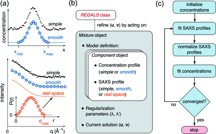
Figure 1.
Overview of the REGALS method. (a) Parametric basis vectors representing concentrations (top panel) and SAXS profiles (bottom panel). In simple vectors, each sample (q or x) is given an independent parameter (black dots). A smooth vector represents the data by linear interpolation between control points (blue circles) over the region of support (x min and x max, top panel). A real-space vector samples the P(r) function (orange circles) up to the maximum particle dimension (d max) and the corresponding SAXS intensities (orange curve) are calculated by Fourier transform [equation (8)]. (b) Experimental restraints are expressed in the software by mixing and matching basis vector types using a flexible object hierarchy. The basis vectors representing SAXS profiles (u) and concentrations (v) are refined by methods in the high-level REGALS class. (c) The refinement algorithm based on regularized ALS. At each iteration, regularized linear least-squares fits are performed on the SAXS profiles [equation (17)] and concentrations [equation (18)] in an alternating fashion until a user-specified convergence test is satisfied.

