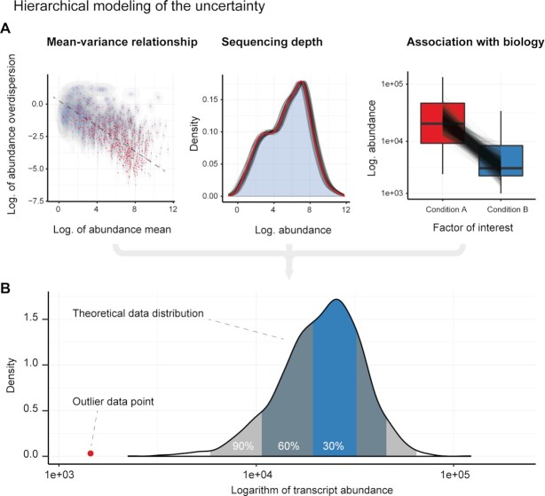
Figure 1.

Graphical example of the estimation of the theoretical data distribution. The theoretical data distribution is estimated for each biological-replicate/transcript pair from the joint posterior distributions. (A) Left: the uncertainty of transcript-wise abundance baseline, where log-overdispersions are modelled in association with their log-mean. The point estimates are coloured in red, while the ellipses represent the 2D credible intervals 40% (blue) and 95% (grey); Middle: the density histogram of the posterior expected values for all genes for one biological replicate, adjusted by the exposure parameter (95% credible interval). The overlapping densities represent the uncertainty of the sequencing depth for one biological-replicate, modelled by the exposure parameter. The red curve corresponds with the adjustment for the mean of the posterior probability of the inferred exposure rate; Right: the uncertainty of the expected abundance values (95% credible interval) of a single transcript across two experimental conditions. The boxplots visualize the observed data distribution, while the black lines visualize the posterior densities of expected abundance according to the linear model. (B) An illustrative example of the theoretical transcript abundance distribution that is estimated for a biological replicate/transcript pair. Shaded regions correspond to central credible intervals of the distribution.