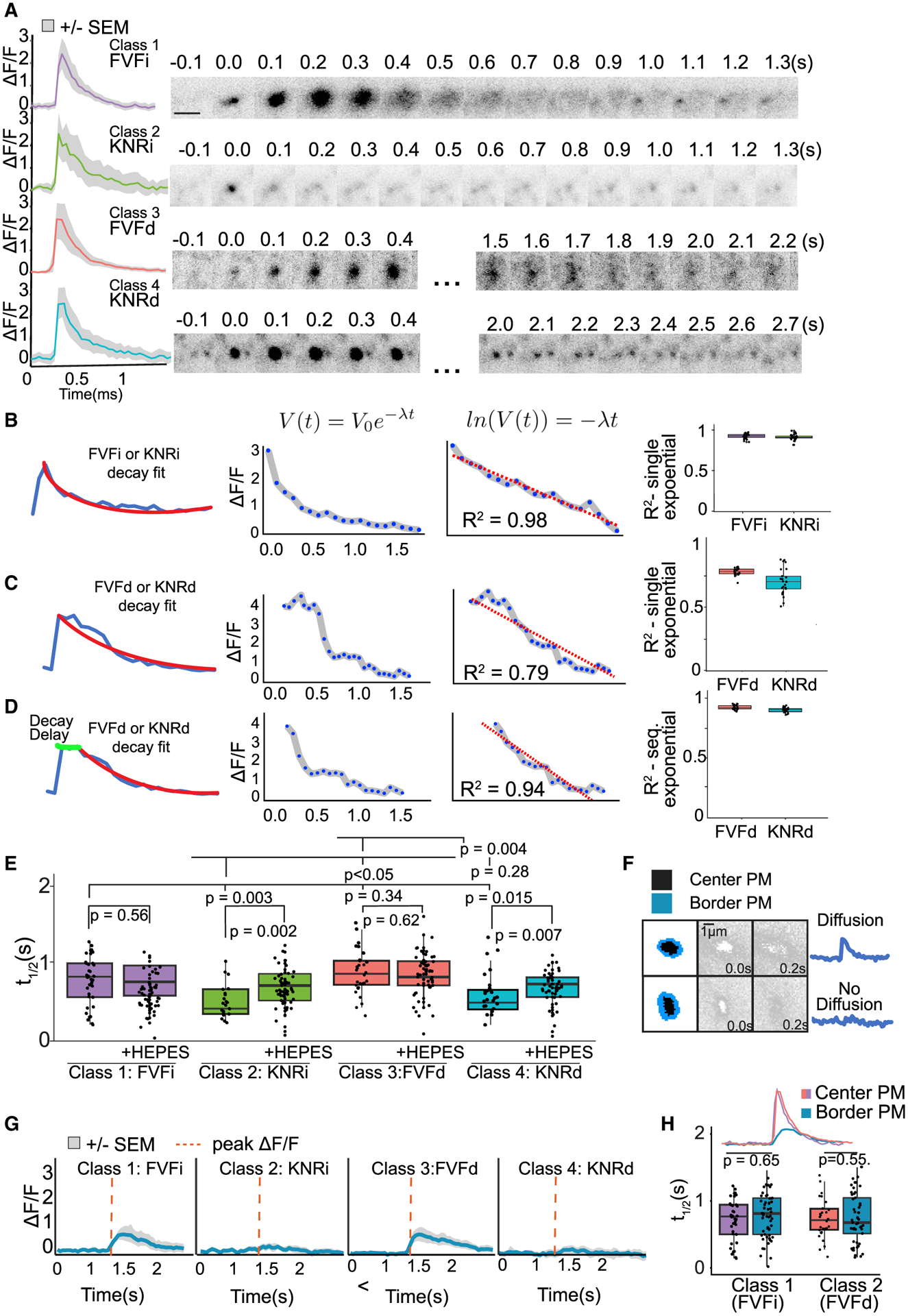
Figure 3. Distinguishing features of four modes of exocytosis.

(A) Mean fluorescent curves ± SEM (gray) and representative images from each class (right).

(B and C) Example single exponential decay fit (V(t) = V₀e^−λt) to class 1 or 2 instantaneous (i) events (B) or to class 3 or 4 delay (d) events (C). The log of an exponential decay curve (ln(V(t)) = −λt) is linear, and the linear regression fit (R²) is an indicator of how good a fit the exponential decay curve is (center graph). Boxplots (right) of R² of class 1 (FVFi) and class 2 (KNRi) events show a good fit (B), whereas fit to class 3 (FVFd) and class 4 (KNRd) is poor.

(D) Sequential exponential decay curves better fit to FVFd and KNRd.

(E) t_1/2 of each class untreated or treated with HEPES. Class 2 and 4 are HEPES sensitive (n = 14 cells per condition; Welch’s t test followed by Benjamini-Hochberg correction).

(F) Schematic of region of exocytic event (black) and bordering PM (blue). Plots of border PM ΔF/F over time demonstrate an event with fluorescence spreading (top, FVF) and an event without (bottom).

(G) Class means ± SEM of ΔF/F in PM bordering exocytic events. Red dotted line indicates peak ΔF/F of center of event.

(H) t_1/2 of fluorescence decay in PM bordering FVFi or FVFd events (border pixels) is not different from the t_1/2 of the exocytic event (center pixels) (n = 14 cells per condition; Welch’s t test).