
FIG. 5.
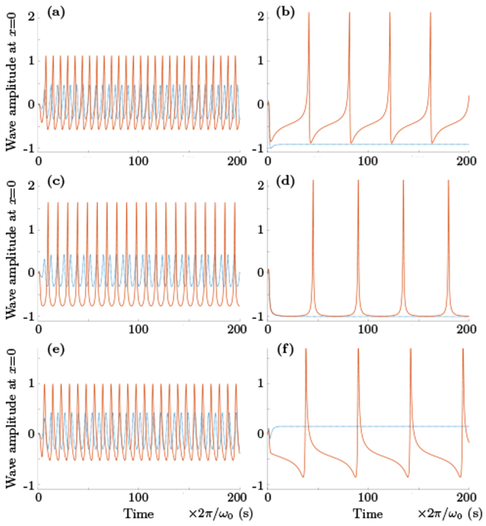
The results of numerical integration of the system (31) and (32), that is time evolution of potential ϕ(x, t) at x = 0 or A(t) cos(B(t) + ωk0t). For all plots the values of ωk0, k0, α and β were set to be equal to 1, δA = 0, and γ and δB were varied. The top,middle and bottom rows show plots for phase delay δB equals to 3π/4, π/2 and π/4 respectively. The left columnn displays transformation from weakly nonlinear oscillations shown by blue dotted lines for γ = 0.75 to more strongly nonlinear regime (solid line, γ = 1.5 (top and bottom) and 2.25 (middle)). The right column shows the strongest nonlinear spiking–like time evolution of potential ϕ (solid line, γ = 2.55 (top and bottom) and 2.96 (middle)) and its transformation to non-oscillatory (blue dotted line) regime for γ = 3 (time and amplitude units are arbitrary).