Optimal Algorithms for Ranked Enumeration of Answers to Full Conjunctive Queries

Abstract

We study ranked enumeration of join-query results according to very general orders defined by selective dioids. Our main contribution is a framework for ranked enumeration over a class of dynamic programming problems that generalizes seemingly different problems that had been studied in isolation. To this end, we extend classic algorithms that find the k-shortest paths in a weighted graph. For full conjunctive queries, including cyclic ones, our approach is optimal in terms of the time to return the top result and the delay between results. These optimality properties are derived for the widely used notion of data complexity, which treats query size as a constant. By performing a careful cost analysis, we are able to uncover a previously unknown trade-off between two incomparable enumeration approaches: one has lower complexity when the number of returned results is small, the other when the number is very large. We theoretically and empirically demonstrate the superiority of our techniques over batch algorithms, which produce the full result and then sort it. Our technique is not only faster for returning the first few results, but on some inputs beats the batch algorithm even when all results are produced.

1. INTRODUCTION

Joins are an essential building block of queries in relational and graph databases, and recent work on worst-case optimal joins for cyclic queries renewed interest in their efficient evaluation [73]. Part of the excitement stems from the fact that conjunctive query (CQ) evaluation is equivalent to other key problems such as constraint satisfaction [61] and hypergraph homomorphism [38]. Similar to [73], we consider full conjunctive queries, yet we are interested in ranked enumeration, recently identified as an important open problem [22]: return output tuples in the order determined by a given ranking function. Here success is measured not only in the time for total result computation, but the main challenge lies in returning the top-ranked result(s) as quickly as possible.

We share this motivation with top-k query evaluation [55], which defines the importance of an output tuple based on the weights of its participating input tuples. However, many top-k approaches, including the famous Threshold Algorithm [36], were developed for a middleware-centric cost model that charges an algorithm only for accesses to external data sources, but does not take into account the cost associated with potentially huge intermediate results. We want optimality guarantees in the standard RAM-model of computation for (1) the time until the first result is returned and (2) the delay between results.

Example 1 (4-cycle query).

Let w be a function that returns the real-valued weight of a tuple and consider 4-cycle query Q_C4 over R₁(A₁, A₂), R₂(A₂, A₃), R₃(A₃, A₄), and R₄(A₄, A₁) with at most n tuples each:

SELECT	R1.A1, R2.A2, R3.A3, R4.A4
FROM	R1, R2, R3, R4
WHERE	R1.A2=R2.A2 AND R2.A3=R3.A3 AND
	R3.A4=R4.A4 AND R4.A1=R1.A1
ORDER BY	w(R1) + w(R2) + w(R3) + w(R4) ASC
LIMIT	k

One can compute the full output with a worst-case optimal join algorithm such as NPRR [73] or Generic-Join [74] and then sort it. Since the fractional edge cover number ρ* of Q_C4 is 2, it takes $\mathcal{O}\left(n^2\right)$ just to produce the full output [9].

On the other hand, the Boolean version of this query (“Is there any 4-cycle?”) can be answered in $\mathcal{O}\left(n^{1.5}\right)$ [69]. Our approach returns the top-ranked 4-cycle in $\mathcal{O}\left(n^{1.5}\right)$ as well. This is remarkable, given that determining the existence of a 4-cycle appears easier than finding the top-ranked 4-cycle (we can use the latter to answer the former). After the top-ranked 4-cycle is found, our approach continues to return the remaining results in ranked order with “minimal” delay.

We develop a theory of optimal ranked enumeration over full CQs. It reveals deeper relationships between recent work that only partially addresses the problem we are considering: Putting aside the focus on twig patterns [26] and subgraph isomorphism [90], graph-pattern ranking techniques can in principle be applied to conjunctive queries. An unpublished paper [33] that was developed concurrently with our work offers a recursive solution for ranked enumeration. All this prior work raises the question of how the approaches are related and whether they can be improved: Can time complexity of the top-k algorithm by Chang et al. [26] be improved for large k and is it possible to extend it to give optimality guarantees for cyclic queries? For [60, 90], how can the worst-case delay be reduced? Is it possible to reduce the complexity of [33] for returning the first few results and can one close the asymptotic gap between the time complexity for returning the top-ranked result and the complexity of the corresponding Boolean query for simple cycles?

It is non-trivial to answer the above questions, because those approaches blend various elements into monolithic solutions, sometimes reinventing the wheel in the process.

Key contributions.

We identify and formally model the underlying structure of the ranked enumeration problem for conjunctive queries and then solve it in a principled way:

1. For CQs that are paths, we identify and formalize the deeper common foundations of problems that had been studied in isolation: k-shortest path, top-k graph-pattern retrieval, and ranked enumeration over joins. While interesting in its own right, uncovering those relationships enables us to propose the first algorithms with optimal time complexity for ranked enumeration of the results of both cyclic and acyclic full CQs. In particular, the top-ranked output tuple of an acyclic join query is returned in time linear in input size. For cyclic queries this complexity increases with the submodular width (subw) of the query [69], which is currently the best known for Boolean queries. Delay between consecutive output tuples is logarithmic in k.

2. To achieve optimality, we make several technical contributions. First, for path CQs we propose a new algorithm Take2 that has lower time complexity for returning the top-k results than all previous work but Eppstein’s algorithm [35], whose practical performance is unknown. Take2 matches the latter and has the added benefit that it can be generalized to arbitrary acyclic queries.¹ Second, to generalize k-shortest path algorithms to arbitrary acyclic CQs, we introduce ranked enumeration over Tree-based Dynamic Programming (T-DP), a variant of Non-Serial Dynamic Programming (NSDP) [20]. Third, we propose Union of T-DP problems (UT-DP), a framework for optimally incorporating in our approach all existing decompositions of a cyclic CQ into a union of trees. Thereby, any decomposition of a full CQ that achieves optimality for the Boolean version of the query will result in an optimal algorithm for ranked enumeration over full CQs in our framework.

3. Ranked enumeration over path CQs forms the backbone of our approach, therefore we analyze all techniques for this problem in terms of both data and query complexity. This is complemented by the first empirical study that directly compares landmark results on ranked enumeration from diverse domains such as k-shortest paths, graph-pattern search, and CQs. Our analysis reveals several interesting insights: (i) In terms of time complexity the best Lawler-type [65] approaches are asymptotically optimal for general inputs and dominate the Recursive Enumeration Algorithm (REA) [33, 57]. (ii) Since REA smartly reuses comparisons, there exist inputs for which it produces the full ordered output with lower time complexity than Lawler; it is even faster than sorting! Our experiments verify this behavior and suggest that Lawler-type approaches should be preferred for small k, but REA for large k. Thus we are the first to not only propose different approaches, but also reveal that neither dominates all others, both in terms of asymptotic complexity and measured running time. (iii) Even though our new Take2 algorithm has lower complexity than Lazy [26], in our environment it is often not the winner because it suffers from higher constant factors.

Further information is available on the project web page at https://northeastern-datalab.github.io/anyk/.

2. FORMAL SETUP

We use ${\mathbb{N}}_i^j$ to denote the set of natural numbers {i, … , j}. For complexity results we use the standard RAM-model of computation that charges $\mathcal{O}(1)$ per data-element access. Reading or storing a vector of i elements therefore costs $\mathcal{O}(i)$ In line with previous work [19, 43, 73], we also assume the existence of a data structure that can be built in linear time to support tuple lookups in constant time. In practice, this is virtually guaranteed by hashing, though formally speaking, only in an expected, amortized sense.

2.1. Conjunctive Queries

Our approach can be applied to any join query, including those with theta-join conditions and projections, but we provide optimality results only for full CQs [73] and hence focus on them. A full CQ is a first-order formula Q(x) = (g₁ ^ · · · ^ g_ℓ), written Q(x) :−g₁(x₁), … , g_ℓ(x_ℓ) in Datalog notation, where each atom g_i represents a relation R_i(x_i) with different atoms possibly referring to the same physical relation, and x = ⋃_i x_i is a set of m attributes. The size of the query |Q| is the size of the formula. We use n to refer to the maximal cardinality of any input relation referenced in Q. Occurrence of the same variable in different atoms encodes an equi-join condition. A CQ can be represented by a hypergraph with the variables as the nodes and the atoms as the hyperedges; acyclicity of the query is defined in terms of the acyclicity of the associated hypergraph [42]. A Boolean conjunctive query just asks for the satisfiability of the formula. We use Q^B to denote the Boolean version of Q. To avoid notational clutter and without loss of generality, we assume that there are no selection conditions on individual relations.

Example 2 (ℓ-path and ℓ-cycle queries).

Let R_i(A, B), $i\in {\mathbb{N}}_1^e$, be tables containing directed graph edges from A to B. A length-ℓ path and a length-ℓ cycle can respectively be expressed as:

$$Q_{P\mathcal{l}}(\text{x}):-R_1\left(x_1,x_2\right),R_2\left(x_2,x_3\right),\dots ,R_{\mathcal{l}}\left(x_{\mathcal{l}},x_{\mathcal{l}+1}\right)$$

$$Q_{C\mathcal{l}}(\text{x}):-R_1\left(x_1,x_2\right),R_2\left(x_2,x_3\right),\dots ,R_{\mathcal{l}}\left(x_{\mathcal{l}},x_1\right).$$

We often represent an output tuple as a vector of those input tuples that joined to produce it, e.g., (r₁, r₂, r₃, r₄) ∈ R₁ × R₂ × R₃ × R₄ for 4-path query Q_P4. We refer to this vector as the result witness.

2.2. Ranked Enumeration Problem

We want to order the results of a full CQ based on the weights of their corresponding witnesses. For maximal generality, we define ordering based on selective dioids [41], which are semirings with an ordering property:

Definition 3 (Semiring). A monoid is a 3-tuple (W, ⊕, $\overline{0}$) where W is a non-empty set, ⊕ : W × W → W is an associative operation, and $\overline{0}$ is the identity element, i.e., $\forall x\in W:x\oplus \overline{0}=\overline{0}\oplus x=x$. In a commutative monoid, ⊕ is also commutative. A semiring is a 5-tuple (W, ⊕, ⊗, $\overline{0}$, $\overline{1}$), where (W, ⊕, $\overline{0}$) is a commutative monoid, (W, ⊗, $\overline{0}$) is a monoid, ⊗ distributes over ⊕, i.e., ∀x, y, z ∈ W : (x ⊕ y)⊗ z = (x ⊗ z) ⊕ (y ⊗ z), and $\overline{0}$ is absorbing for ⊗, i.e., $\forall a\in W:a\otimes \overline{0}=\overline{0}\otimes a=\overline{0}$.

Definition 4 (Selective Dioid). A selective dioid is a semiring for which ⊕ is selective, i.e., it always returns one of the inputs: ∀x, y ∈ W : (x ⊕ y = x) ∨ (x ⊕ y = y).

Note that ⊕ being selective induces a total order on W by setting x ≤ y iff x ⊕ y = x. We define result weight as an aggregate of input-tuple weights using ⊗:

Definition 5 (Tuple Weights). Let w be a weight function that maps each input tuple to some value in W and let Q(x) :− R₁(x₁), … , R_ℓ(x_ℓ) be a full CQ. The weight of a result tuple r is the weight of its witness (r₁, … , r_ℓ), r_i ∈ R_i, $i\in {\mathbb{N}}_1^{\mathcal{l}}$, defined as w(r) = w(r₁) ⊗ · · · w(r_ℓ).

Recall Example 1 where we rank output tuples by the sum of the weights of the corresponding input tuples, i.e., the weight of (r₁, … , r_ℓ) is ${\sum }_{i=1}^{\mathcal{l}}w\left(r_i\right)$. We achieve this by using the selective dioid (${ℝ}^{\infty }$, min, +, ∞, 0) with ${ℝ}^{\infty }=ℝ\cup \left\{\infty \right\}$ that is also called the tropical semiring.

The central problem in this paper is the following:

Definition 6 (Ranked Enumeration). Given a query Q over an input database D, selective dioid (W, ⊕, ⊗, $\overline{0}$, $\overline{1}$), and weight function w as defined above, a ranked enumeration algorithm returns the output of Q on D according to the total order induced by ⊕.

We refer to algorithms for ranked enumeration over the results of a CQ as any-k algorithms. This conforms to our previous work [90] and reflects the fact that the number of returned results need not be set apriori.

Generality.

Our approach supports any selective dioid, including less obvious cases such as lexicographic ordering where two output tuples are first compared on their R₁ component, and if equal then on their R₂ component, and so on. For this to be well-defined, there must be a total order on the tuples within each relation. Without loss of generality, assume this total order is represented by the natural numbers, such that input tuple r has weight $w^{\prime }(r)\in \mathbb{N}$. For the selective dioid, we set $W={\mathbb{N}}^{\mathcal{l}}$, i.e., each tuple weight is an ℓ-dimensional vector of integers. Input tuple r_j ∈ R_j has weight w(r_j) = (0, … , 0, w′(r_j), 0, … , 0) with zeros except for position j that stores the “local” weight value in R_j. Operator ⊗ is standard element-wise vector addition, therefore the weight of a result tuple with witness (r₁, … , r_ℓ) is (w′(r₁), … , w′(r_ℓ)). To order two such vectors, ⊕ implements element-wise minimum, e.g., for ℓ = 2, (a, b) ⊕ (c, d) = (a, b) iff w′(a) < w′(c) or w′(a) = w′(c) and w′(b) < w′(d). The $\overline{0}$ and $\overline{1}$ elements of the dioid are ℓ-dimensional vectors (∞, … , ∞) and (0, … , 0), respectively.

We will present our approach for the tropical semiring (${ℝ}^{\infty }$, min, +, ∞, 0). Generalization to other selective dioids follows immediately from the fact that the only algebraic properties that are used in our derivations are those mentioned in Definitions 3 and 4. Note that addition over real numbers has an inverse, hence (${ℝ}^{\infty }$, +, 0) is a group, not just a monoid. This simplifies the algorithm somewhat, but our main result (Theorem 13) holds even without the inverse with some minor subtleties (see the full version [87]).

2.3. Determining Optimality

An any-k algorithm should return the first result as soon as possible, then the next results with minimal delay. We therefore ask “how long does it take to return the k top-ranked results, for any value of k?” and use TT(k) and MEM(k) to denote time and space complexity, respectively, to produce the k top results. We will pay particular attention to the special cases of time-to-first (TTF = TT(1)) and time-to-last (TTL = TT(|out|)), where out denotes the output of the query. In line with most previous work on worst-case optimal join algorithms and decompositions of cyclic queries, we measure asymptotic cost in terms of data complexity [88], i.e., treat query size |Q| as a constant. The exception is the in-depth analysis of ranked enumeration algorithms for path CQs (Section 4.3), where including query complexity reveals interesting differences.

Consider full CQ Q over input relations with at most n tuples. It takes $\mathcal{O}(n)$ just to look at each input tuple and $\mathcal{O}(k)$ to output k result tuples, establishing Ω(n + k) as a lower bound for TT(k). Since we also require the output to be sorted and sorting k items has complexity Ω(k log k), we consider a ranked enumeration algorithm to be optimal if it satisfies $\text{TT}(k)=\mathcal{O}(n+k\text{ log }k)$.² For acyclic CQs, this TT(k) optimality target is realistic, because the well-known Yannakakis algorithm [92] computes the full (unsorted) output in time $\mathcal{O}(n+\mid \text{out}\mid )$.

For cyclic CQs, Ngo et al. [73] argue that the join result cannot be computed in $\mathcal{O}(n+\mid \text{out}\mid )$ and propose the notion of worst-case optimal (WCO) join algorithms, whose computation time is $\mathcal{O}\left(n+\mid {\text{out}}_{\text{WC}}\mid \right)$. Here, |out_WC| is the maximum output size of query Q over any possible database instance, which is determined by the AGM bound [9]. WCO join algorithms are thus not sensitive to the actual output size of the query on a given database instance. Abo Khamis et al. [5] argue for a stronger, output-sensitive notion of optimality based on the width ω of a decomposition of a cyclic CQ Q into a set $\overline{Q}$ of acyclic CQs covering Q.³ The input relations of the acyclic CQs in $\overline{Q}$ are derived from the original input and have cardinality $\mathcal{O}\left(n^{\omega }\right)$ for ω ≥ 1 ideally as small as possible. Let $\mathcal{A}$ be such a decomposition-based algorithm and let $T(\mathcal{A})$ denote its time complexity for creating decomposition $\overline{Q}$. By applying the Yannakakis algorithm to the acyclic queries in $\overline{Q}$, cyclic query Q can be evaluated in time $\mathcal{O}(T(\mathcal{A})+\mid \text{out}\mid )$ and its Boolean version Q^B in $\mathcal{O}(T(\mathcal{A}))$. The current frontier are decompositions based on the submodular width ω = subw(Q) [69], which is considered a yardstick of optimality for full and Boolean CQs [5].

We adopt this notion of optimality and, arguing similar to the acyclic case, we say that ranked enumeration over a full CQ is optimal if $\text{TT}(k)=\mathcal{O}(T(\mathcal{A})+k\text{log}k)$. Intuitively, this ensures that ranked enumeration adds “almost no overhead” compared to unranked enumeration, because outputting k results would take at least Ω(k).

3. PATH QUERY AND ITS CONNECTION TO DYNAMIC PROGRAMMING (DP)

We formulate optimal ranked enumeration for path queries as a Dynamic Programming (DP) problem, then generalize to trees and cyclic queries. Following common terminology, we use DP to denote what would more precisely be called deterministic serial DP with a finite fixed number of decisions [21, 29, 30]. These problems have a unique minimum of the cost function and DP constructs a single solution that realizes it. Formally, a DP problem has a set of states S, which contain local information for decision-making [21]. We focus on what we will refer to as multi-stage DP. Here each state belongs to exactly one of ℓ > 0 stages, where S_i denotes the set of states in stage i, $i\in {\mathbb{N}}_0^{\mathcal{l}}$. The start stage has a single state S₀ = {s₀} and there is a terminal state s_ℓ+1 which we also denote by t for convenience. At each state s of stage i, we have to make a decision that leads to a state s′ ∈ S_i+1. We use $E\subseteq {\cup }_{i=0}^{\mathcal{l}}\left(S_i\times S_{i+1}\right)$ for the set of possible decisions.

DP is equivalent to a shortest-path problem on a corresponding weighted graph, in our case a (ℓ + 2)-partite directed acyclic graph (DAG) [21, 30], where states correspond to nodes and decisions define the corresponding edges. Each decision (s, s′) is associated with a cost w(s, s′), which defines the weight of the corresponding edge in the shortest-path problem.⁴ By convention, an edge exists iff its weight is less than ∞.

We now generalize the path definition from Example 2 and show that ranked enumeration over this query can be modeled as an instance of DP. Consider

$$Q_{P\mathcal{l}}^{\prime }(\text{x},\text{y}):-R_1\left({\text{y}}_1,{\text{x}}_2\right),R_2\left({\text{x}}_2,{\text{y}}_2,{\text{x}}_3\right),\dots ,R_{\mathcal{l}}\left({\text{x}}_{\mathcal{l}},{\text{y}}_{\mathcal{l}},{\text{x}}_{\mathcal{l}+1}\right),$$

allowing multiple attributes in the equi-join conditions and additional attribute sets y_i that do not participate in joins. This query can be mapped to a DP instance as follows: (1) atom R_i corresponds to stage S_i and each tuple in R_i maps to a unique state in S_i, (2) there is an edge between s ∈ S_i and s′ ∈ S_i+1 iff the corresponding input tuples join and the edge’s weight is the weight of the tuple corresponding to s′, (3) there is an edge from s₀ to each state in S₁ whose weight is the weight of the corresponding R₁-tuple, and (4) each state in S_ℓ has an edge to t of weight 0. Clearly, there is a 1:1 correspondence between paths from s₀ to t and output tuples of Q′_Pℓ, and path “length” (weight) equals output-tuple weight. Hence the k-th heaviest output tuple corresponds to the k-shortest path in the DP instance.

Example 7 (Cartesian Product).

We use the problem of finding the minimum-weight output of Cartesian product R₁ × R₂ × R₃ as the running example. Let R₁ = {“1”, “2”, “3”}, R₂ = {“10”, “20”, “30”} and R₃ = {“100”, “200”, “300”} and set tuple weight equal to tuple label, e.g., tuple “20” in R₂ has weight w(“20”) = 20. Fig. 1 depicts how this problem translates into our framework.

Figure 1:

DP instance for Example 7.

A solution to the DP problem is a sequence of ℓ states Π = 〈s₁ … s_ℓ〉 that is admissible, i.e. (s_i, s_i+1) ∈ E, $\forall i\in {\mathbb{N}}_0^{\mathcal{l}}$. The objective function is the total cost of a solution,

$$w(\Pi )=\sum _{i=0}^{\mathcal{l}}w\left(s_i,s_{i+1}\right),$$ (1)

and DP finds the minimal-cost solution Π₁. The index denotes the rank, i.e., Π_k is the k-th best solution.

Principle of optimality.

[15, 16] The core property of DP is that a solution can be efficiently derived from solutions to subproblems. In the shortest-path view of DP, the subproblem at any state s ∈ S_i is the problem of finding the shortest path from s to t. With Π₁(s) and π₁(s) denoting the shortest path from s and its weight respectively, DP is recursively defined for all states s ∈ S_i, $i\in {\mathbb{N}}_0^{\mathcal{l}+1}$ by

$$\begin{gathered} {\pi }_1(s)=0\text{ for terminal }s\in S_{\mathcal{l}+1} \\ {\pi }_1(s)=\underset{{}_{\left(s,s^{\prime }\right)\in E}}{\text{min}}\left\{w\left(s,s^{\prime }\right)+{\pi }_1\left(s^{\prime }\right)\right\},\text{ for }s\in S_i,i\in {\mathbb{N}}_0^{\mathcal{l}}. \end{gathered}$$ (2)

The optimal DP solution is π₁(s₀), i.e., the weight of the lightest path from s₀ to t. For convenience we define the set of optimal paths reachable from s according to Eq. (2) as Choices₁(s) = {s ◦ Π₁(s′) | (s, s′) ∈ E}. Here ◦ denotes concatenation, i.e., s_i ◦ 〈s_i+1 … s_ℓ〉 = 〈s_i s_i+1 … s_ℓ〉.

Example 8 (continued).

Consider state “2” in Fig. 2. It has three outgoing edges and π₁(“2”) is computed as the minimum over these three choices. The winner is path “2” ◦ Π₁(“10”) of weight 112. Similarly, Π₁(“10”) is found as “10” ◦ Π₁(“100”), and so on.

Figure 2:

Excerpt from Fig. 1, showing Choices₁(s) for some states s. Term s ◦ Π₁(s′) : w denotes a choice, which is a path from s, and its weight w = w(s, s′) + π₁(s′).

Equation (2) can be computed for all states in time $\mathcal{O}(\left|S\right|+\left|E\right|)$ bottom-up, i.e., in decreasing stage order from ℓ + 1 to 0. Consider stage S_i: To compute Choices₁(s) for state s ∈ S_i, the algorithm retrieves all edges (s, s′) ∈ E from s to any state s′ ∈ S_i+1, looks up π₁(s′), and keeps track of the minimal total weight w(s, s′) + π₁(s′) on-the-fly. (If no such edge is found, then the weight is set to ∞.) When computing π₁(s), the algorithm also adds pointers to keep track of optimal solutions. E.g., in Fig. 2 entry “2” ◦ Π₁(“30”) at state “2” would point to the minimum-weight choice “30” ◦ Π₁(“100”) at state “30”. This way the corresponding paths can be reconstructed by tracing the pointers back “top-down” from π₁(s₀) [21]. Notice that DP needs only the pointer from the top choice at each state, but adding the others is “free” complexity-wise, which we later use for ranked enumeration.

Whenever the bottom-up phase determines π₁(s) = ∞ during the evaluation of Eq. (2), then that state s and all its adjacent edges can be removed without affecting the space of solutions. We use ${\mathbb{S}}_i\subseteq S_i$ and $\mathbb{E}\subseteq E$ to denote the remaining sets of states and decisions, respectively. This DP algorithm corresponds to variable elimination [31] on the tropical semiring [39, 78] and is reminiscent of the semi-join reductions by Yannakakis [92], which corresponds to DP with variable elimination on the Boolean semiring [2].

Encoding equi-joins efficiently.

For an equi-join, the shortest-path problem has $\mathcal{O}(\mathcal{l}n)$ states and $\mathcal{O}\left(\mathcal{l}{n}^2\right)$ edges, therefore the DP algorithm has quadratic time complexity in the number of tuples. We reduce this to $\mathcal{O}(\mathcal{l}n)$ by an equi-join specific graph transformation illustrated in Fig. 3. Consider the join between R₁ and R₂, representing stages S₁ and S₂, respectively. For each join-attribute value, the corresponding states in R₁ and R₂ form a fully connected bipartite graph. For each state, all incoming edges have the same weight, as edge weight is determined by tuple weight. Hence we can represent the subgraph equivalently with a single node “in-between” the matching states in S₁ and S₂, assigning zero weight to the edges adjacent to states in S₁ and the corresponding tuple weight to those adjacent to a state in S₂. The transformed representation has only $\mathcal{O}(\mathcal{l}n)$ edges. At its core, our encoding relies on the conditional independence of the non-joining attributes given the join attribute value, a property also exploited in factorized databases [75]. Here we provide a different perspective on it as a graph transformation that preserves all paths.

Figure 3:

Equi-join from $\mathcal{O}\left(n^2\right)$ representation to $\mathcal{O}(n)$.

4. ANY-K ALGORITHMS FOR DP

We defined a class of DP problems that can be described in terms of a multi-stage DAG, where every solution is equivalent to a path from s₀ to t in graph $\left(\mathbb{S}={\cup }_{i=0}^{\mathcal{l}+1}{\mathbb{S}}_i,\mathbb{E}\right)$. Hence we use terminology from DP (solution, state, decision) and graphs (path, node, edge) interchangeably.

In addition to the minimum-cost path, ranked enumeration must retrieve all paths in cost order. Let Π_k(s) be the k^th-shortest path from s to t and π_k(s) its cost. The asymptotically best k-shortest-paths algorithm was proposed by Eppstein [35], yet it is not the best choice for our use case. In the words of its author, it is “rather complicated”, thus it is unclear how to extend it from path to tree queries. Since our DP problems are only concerned with multi-stage DAGs (Eppstein targets more general graphs), we propose a simpler and easier-to-extend algorithm, Take2, that guarantees the same complexity as Eppstein.⁵

Below we explore algorithms that fall into two categories. The first appeared in various optimization contexts as methods that partition the solution space and trace their roots to Lawler [65] and Murty [70], including recent work on subgraph isomorphism [26]. We call this family anyK-part; it includes Take2. The second finds the k-shortest paths in a graph via recursive equations [34, 57]. We refer to the application of this idea to our framework as anyK-rec.

4.1. Repeated Partitioning DP (ANYK-PART)

4.1.1. The Lawler Procedure and DP

Lawler [65] proposed a procedure for ranked enumeration by repeatedly partitioning the solution space, which can be applied to any optimization problem over a fixed set of variables, not only DP. In our problem, there is one variable per stage and it can take any state in that stage as a value. Lawler only assumes the existence of a method best that returns the optimal variable assignment over any space $S_1^{\prime }\times \cdots \times S_{\mathcal{l}}^{\prime }$, where $\forall i:S_i^{\prime }\subseteq S_i$.

The top-ranked solution $s_1^{*}\dots s_{\mathcal{l}}^{*}$ is obtained by executing best on the unconstrained space S₁ × · · · × S_ℓ. To find the second-best solution, Lawler creates ℓ disjoint subspaces such that subspace i has the first i−1 variables fixed to the top-ranked solution’s prefix $\langle s_1^{*}\dots s_{i-1}^{*}\rangle$ and the i-th variable restricted to $S_i-\left\{s_i^{*}\right\}$. Then it applies best to each of these subspaces to find the top solution in each. The second-best overall solution is the best of these ℓ subspace solutions. The procedure continues analogously by generating the corresponding subspaces for the second-best solution, adding them to a priority queue of candidates.

Chang et al. [26] showed that the k^th-ranked solution 〈s₁ … s_ℓ〉 is the output of best on some subspace

$$P=\left\{s_1\right\}\times \cdots \times \left\{s_{r-1}\right\}\times \left(S_r-U_r\right)\times S_{r+1}\times \cdots \times S_{\mathcal{l}},$$ (3)

with U_r being a set of states excluded from S_r. The new candidates to be added to the candidate set for the (k + 1)^st result are the results obtained by executing best on the following ℓ − r + 1 subspaces:

$$\begin{gathered} P=\left\{s_1\right\}\times \cdots \times \left\{s_{r-1}\right\}\times \left(S_r-U_r\right)\times S_{r+1}\times \cdots \times S_{\mathcal{l}}, \\ {P}_r=\left\{s_1\right\}\times \cdots \times \left\{s_{r-1}\right\}\times \left(S_r-U_r-\left\{s_r\right\}\right)\times S_{r+1}\times \cdots \times S_{\mathcal{l}} \\ ⋮ \\ {P}_{\mathcal{l}}=\left\{s_1\right\}\times \cdots \times \left\{s_{r-1}\right\}\times \cdots \times \left\{s_{\mathcal{l}-1}\right\}\times \left(S_{\mathcal{l}}-\left\{s_{\mathcal{l}}\right\}\right), \end{gathered}$$

Efficient computation.

Instead of calling best from scratch on each subspace, we propose to exploit the structure of DP. Consider any subspace P as defined in Eq. (3). Since prefix 〈s₁ … s_r−1〉 is fixed, we need to find the best suffix starting from state s_r−1. In the next stage S_r, only states that are not in exclusion set U_r can be selected, i.e., the set of choices at s_r−1 is restricted by U_r. Formally,

$$\text{best}(P)=s_1\dots s_{r-1}s\circ {\Pi }_1(s),\text{ where}$$ (4)

$$s=\text{arg }\underset{s^{\prime }\in S_r-U_r}{\text{min}}\{w\left(s_{r-1},s^{\prime }\right)+{\pi }_1\left(s^{\prime }\right)\mid s_{r-1}\circ {\Pi }_1\left(s^{\prime }\right)\in {\text{ Choices}}_{\text{1}}\left(s_{r-1}\right)\},$$ (5)

therefore Eq. (5) can be solved using only information that was already computed by the standard DP algorithm. Note that all elements in a choice set other than the minimum-weight element are often referred to as deviations from the optimal path.

Example 9 (Continued).

After returning Π₁(s₀) = 〈“1” “10” “100”〉, Lawler would solve three new optimization problems to find the second-best result. The first subspace is the set of paths that start at s₀, but cannot use state “1”. The second has prefix 〈“1”〉 and cannot use state “10”. The third has prefix 〈“1” “10” 〉 and cannot use state “100”. The best solution to the first subproblem is 〈“2” “10” “100”〉, corresponding to deviation s₀ ◦ π₁(“2”) of weight 112. For the second subproblem, the best result is found similarly as the second-best option “1” ◦ π₁(“20”) = 〈“1” “20” “100”〉. For the third subproblem, the best sub space solution 〈“1” “10” “200”〉 is obtained analogously at state “10”

4.1.2. The ANYK-PART family of algorithms

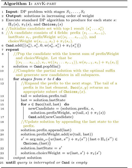
We propose a generic template for anyK-part algorithms and show how all existing approaches and our novel Take2 algorithm are obtained as specializations based on how the Lawler-created subspace candidates are managed. All anyK-part algorithms first execute standard DP, which produces for each state s the shortest path Π₁(s), its weight π₁(s), and set of choices Choices₁(s). The main feature of anyK-part is a set Cand of candidates: it manages the best solution(s) found in each of the subspaces explored so far. To produce the next result, the anyK-part algorithm (Algorithm 1) (1) removes the lightest candidate from the candidate set Cand, (2) expands it into a complete solution, and (3) adds all new candidates found in the corresponding subspaces to Cand. We implement Cand using a priority queue with combined logarithmic time for removing the top element and inserting a batch of new candidates.

Example 10 (continued).

The standard DP algorithm identifies 〈“1” “10” “100”〉 as the shortest path and generates the choice sets as shown in Fig. 2. Hence Cand initially contains only candidate (〈s₀〉, “1”, 0, 1 + 110 = 111) (Line 6), which is popped in the first iteration of the repeat-loop (Line 7), leaving Cand empty for now. The for-loop (Line 11) is executed for stages 1 to ℓ = 3. For stage 1, we have tail = s₀ and last = “1”. For the successor function (Line 15), there are different choices as we discuss in more detail in Section 4.1.3. For now, assume Succ(x, y) returns the next-best choice at state x after the previous choice y. Hence the successor of “1” at state s₀ is “2”. As a result, newCandidate is set to ((〈s₀〉, “2”, 0, 2 + 110)—it is the winner for the first subspace—and added to Cand. Then the solution is expanded (Line 19) to (〈s₀ “1”〉, “10”, 1, 10 + 100), because “10” is the best choice from “1”. The next iteration of the outer for-loop (Line 11) adds candidate (〈s₀ “1”〉, “20”, 1, 20 + 100) to Cand and updates the solution to (〈s₀ “1” “10”〉, “100”, 11, 100). The third and final iteration adds candidate (〈s₀ “1” “10” 〉, “200”, 11, 200) and updates the solution to (〈s₀ “1” “10” “100”〉, t, 111, 0), which is returned as the top-1 result.

At this time, Cand contains entries (〈s₀〉, “2”, 0, 112), (〈s₀ “1”〉, “20”, 1, 120), and (〈s₀ “1” 10” 〉, “200”, 11, 200). Note that each is the shortest path in the corresponding subspace as defined by the Lawler procedure. Among the three, (〈s₀〉, “2”, 0, 112) is popped next, because it has the lowest sum of prefix-weight (0) and choice-weight (112). The first new candidate created for it is (〈s₀〉, “3”, 0, 113), followed by (〈s₀ “2”〉, “20”, 2, 120), and (〈s₀ “2” “10”〉, “200”, 12, 200). At the same time, the solution is expanded to (〈s₀ “2” “10” “100”〉, t, 112, 0).

4.1.3. Instantiations of ANYK-PART

The main design decision in Algorithm 1 is how to manage the choices at each state and how to implement successor-finding (Line 15) over these choices.

Strict approaches.

A natural implementation of the successor function returns precisely the next-best choice.

Eager Sort (Eager):

Since a state might be reached repeatedly through different prefixes, it may pay off to pre-sort all choice sets by weight and add pointers from each choice to the next one in sort order. Then Succ(x, y) returns the next-best choice at x in constant time by following the next-pointer from y.

Lazy Sort (Lazy):

For lower pre-processing cost, we can leverage the approach Chang et al. [26] proposed in the context of graph-pattern search. Instead of sorting a choice set, it constructs a binary heap in linear time. Since all but one of the successor requests in a single repeat-loop execution are looking for the second-best choice⁶, the algorithm already pops the top two choices off the heap and moves them into a sorted list. For all other choices, the first access popping them from the heap will append them to the sorted list that was initialized with the top-2 choices. As the algorithm progresses, the heap of choices gradually empties out, filling the sorted list and thereby converging to Eager.

Relaxed approaches.

Instead of finding the single true successor of a choice, what if the algorithm could return a set of potential successors? Correctness is guaranteed, as long as the true successor is contained in this set or is already in Cand. (Adding potential successors early to Cand does not affect correctness, because they have higher weight and would not be popped from Cand until it is “their turn.”) This relaxation may enable faster successor finding, but inserts candidates earlier into Cand.

All choices (All):

This approach is based on a construction that Yang et al. [90] proposed for any-k queries in the context of graph-pattern search. Instead of trying to find the true successor of a choice, all but the top choice are returned by Succ. While this avoids any kind of pre-processing overhead, it inserts $\mathcal{O}(n)$ potential successors into Cand.

Take2:

We propose a new approach that has better asymptotic complexity than any of the above. Intuitively, we want to keep pre-processing at a minimum (like All), but also return a few successors fast (like Eager). To this end, we organize each choice set as a binary heap. In this tree structure, the root node is the minimum-weight choice and the weight of a child is always greater than its parent. Function Succ(x, y) (Line 15) returns the two children of y in the tree. Unlike Lazy, we never perform a pop operation and the heap stays intact for the entire operation of the algorithm; it only serves as a partial order on the choice set, pointing to two successors every time it is accessed. Also note that the true successor does not necessarily have to be a child of node y. Overall, returning two successors is asymptotically the same as returning one and heap construction time is linear [29], hence this approach asymptotically dominates the others.

4.2. Recursive Enumeration DP (ANYK-REC)

anyK-rec relies on a generalized principle of optimality [68]: if the k-th path from start node s₀ goes through $s\in {\mathbb{S}}_1$ and takes the j_s-lightest path Π_js(s) from there, then the next lightest path from s₀ that goes through s will take the (j_s + 1)-lightest path Π_js+1(s) from there. We will refer to the prototypical algorithm in this space as Recursive [57]. Recall that lightest path Π₁(s₀) from start node s₀ is found as the minimum-weight path in Choices₁(s₀). Assume it goes through $s\in {\mathbb{S}}_1$. Through which node does the 2^nd-lightest path Π₂(s₀) go? It has to be either the 2^nd-lightest path through s, of weight w(s₀, s) + π₂(s), or the lightest path through any of the other nodes adjacent to s₀. In general, the k-th lightest path Π_k(s₀) is determined as the lightest path in some later version ${\text{Choices}}_k\left(s_0\right)=\left\{s_0\circ {\Pi }_{j_s}(s)\mid \left(s_0,s\right)\in \mathbb{E}\right\}$ of the set of choices, for appropriate values of j_s. Let ${\Pi }_k\left(s_0\right)=s_0\circ {\Pi }_{j_{s^{\prime }}}\left(s^{\prime }\right)$. Then the (k + 1)^st solution Π_k+1(s₀) is found as the minimum over the same set of choices, except that $s_0\circ {\Pi }_{j_{s^{\prime }+1}}\left(s^{\prime }\right)$ replaces $s_0\circ {\Pi }_{j_{s^{\prime }}}\left(s^{\prime }\right)$. To find ${\Pi }_{j_{s^{\prime }+1}}\left(s^{\prime }\right)$, the same procedure is applied recursively at s′ top-down. Intuitively, an iterator-style next call at start node s₀ triggers a chain of ℓ such next calls along the path that was found in the previous iteration.

Example 11 (continued).

Consider node “2” in Fig. 1. Since it has adjacent states “10”, “20”, and “30” in the next stage, the lightest path Π₁(“2”) is selected from Choices₁(“2”) = {“2” ◦ Π₁(“10”), “2” ◦ Π₁(“20”), “2” ◦ Π₁(“30”)} as shown in Fig. 2. The first next call on state “2” returns “2” ◦ Π₁(“10”), updating the set of choices for Π₂(“2”) to {“2” ◦ Π₂(“10”), “2” ◦ Π₁(“20”), “2” ◦ Π₁(“30”)} as shown in the left box in Fig. 4. The subsequent next call on state “2” then returns “2” ◦ Π₁(“20”) for Π₂(“2”), causing “2” ◦ Π₁(“20”) in Choices₂(“2”) to be replaced by “2” ◦ Π₂(“20”) for Choices₃(“2”); and so on.

Figure 4:

Example 11: Recursive enumeration at state “2”.

As the lower-ranked paths starting at various nodes in the graph are computed, each node keeps track of them for producing the results as shown in Fig. 5. For example, the pointer from Π ₁(“2”) to Π₁(“10”) at node “10” was created by the first next call on “2”, which found “2” Π₁(“10”) as the lightest path in the choice set. For details see [87].

Figure 5:

Pointers between solutions from and to “2”.

4.3. Any-k DP Algorithm Complexity

In contrast to the discussion in Section 2.3, which focused on data complexity and treated query size as a constant, we now include query size in the analysis to uncover more subtle performance tradeoffs between the different any-k approaches. Since each input relation has at most n tuples, the DP problem has $\mathcal{O}(\mathcal{l}n)$ nodes, each with at most n outgoing edges. Based on our equi-join construction (Fig. 3), it is easy to see that the total number of edges is $\left|E\right|=\mathcal{O}(\mathcal{l}n)$. For simplicity we make the following assumptions: (1) the maximum arity of a relation is bounded by a constant, thus |Q| = ℓ, and (2) the operations ⊕ and ⊗ of the selective dioid over which the ranking function is defined take $\gamma =\mathcal{O}(1)$ time to execute. It is straightforward to extend our analysis to scenarios where those assumptions do not hold. Note that (2) holds for many practical problems, e.g., tropical semiring (${ℝ}^{\infty }$, min, +, ∞, 0), but not for lexicographic ordering where weights are ℓ-dimensional vectors and hence $\gamma =\mathcal{O}(\mathcal{l})$. With Batch, we refer to an algorithm that sorts the full output produced by the Yannakakis algorithm [92].

4.3.1. Time to First

All any-k algorithms first execute DP to find the top result and create all choice sets in time $\mathcal{O}(\mathcal{l}n)$. Eager requires $\mathcal{O}(\mathcal{l}n\text{ log }n)$ for sorting of choice sets. Heap construction for Lazy and Take2 takes time linear in input size.

4.3.2. Delay

Each algorithm requires $\mathcal{O}(\mathcal{l})$ to assemble an output tuple. In addition, the following costs are incurred:

anyK-rec.

In Recursive each next call on s₀ triggers $\mathcal{O}(\mathcal{l})$ next calls in later stages—at most one per stage. The call deletes the top choice at the state and replaces it with the next-heavier path through the same child node in the next stage (see Fig. 4). With a priority queue, these operations together take time $\mathcal{O}(\text{log }n)$ per state accessed, for a total delay of $\mathcal{O}(\mathcal{l}\text{ log }n)$ between consecutive results. In total, it takes $\mathcal{O}(\mathcal{l}n+k\mathcal{l}\text{ log }n)$ produce the top k results. The resulting TTL bound of $\mathcal{O}(\mathcal{l}n+\mid \text{out}\mid \cdot \mathcal{l}\text{ log }n)$ can be loose because it does not take into account that in later iterations many next calls will stop early because the corresponding suffixes Π_i had already been computed by an earlier call:

Theorem 12. There exist DP problems where Recursive has strictly lower TTL complexity than Batch.

An example are problems with near-worst-case output size Θ(n^ℓ) such as the Cartesian product [87]. The lower TTL of Recursive is at first surprising, given that Batch is optimized for bulk-computing and bulk-sorting the entire output. Intuitively, Recursive wins because it exploits the multi-stage structure of the graph—which enables the re-use of shared path suffixes—while Batch uses a general-purpose comparison-based sort algorithm. We leave as future work a more precise characterization of graph properties that ensure better TTL for Recursive over Batch.

anyK-part.

For all anyK-part algorithms, popMin and bulk-insertion of all new candidates during result expansion take $\mathcal{O}(\text{log}\mid \text{Cand}\mid )$. For efficient candidate generation (Line 15 in Algorithm 1) the new candidates do not copy the solution prefix, but simply create a pointer to it. Therefore, a new candidate is created in $\mathcal{O}(1)$.

Eager finds each successor in constant time. Since |Cand| ≤ kℓ, its total delay is $\mathcal{O}(\text{log}(k\mathcal{l})+\mathcal{l})=\mathcal{O}(\text{ log }k+\mathcal{l})$. For Lazy, in the first iteration of the main for-loop (Algorithm 1, Line 11), finding the successor (Line 15) requires at most one pop on a heap storing $\mathcal{O}(n)$ choices. All later iterations find the successor in constant time. Hence total delay is $\mathcal{O}(\text{log }k+\mathcal{l}+\text{log }n)$. The All algorithm might insert up to ℓn new candidates to Cand for each result produced. Hence access to Cand after producing k results takes a total of $\mathcal{O}(\text{log}(k\mathcal{l}n))$. All together, delay is $\mathcal{O}(\text{log }k+\text{log }\mathcal{l}+\text{log }n+\mathcal{l}n)=\mathcal{O}(\text{log }k+\mathcal{l}n)$. Finally, Take2 finds up to two successor candidates of a choice in constant time. Delay therefore is $\mathcal{O}(\text{log }k+\mathcal{l})$. It is easy to see that all these algorithms have worst-case TTL of $\mathcal{O}\left(n^{\mathcal{l}}\cdot \mathcal{l}\text{ log }n\right)$, the same as Batch (refer to [90] for All).

4.3.3. Memory

All algorithms need $\mathcal{O}(\mathcal{l}n)$ memory for storing the input. The memory consumption of anyK-part approaches depends on the size of Cand. All grows Cand by $\mathcal{O}(\mathcal{l}n)$ elements in each iteration, but creates at most |out| candidates in total. The others create only $\mathcal{O}(\mathcal{l})$ new candidates per iteration, thus $\text{MEM}(k)=\mathcal{O}(\mathcal{l}n+k\mathcal{l})$. For Recursive, size of a choice set Choices_k(s) is bounded by the out-degree of s, hence cannot exceed n. However, we need to store the suffixes Π_i(s) produced by the algorithm, whose number is $\mathcal{O}(\mathcal{l})$ per iteration, thus MEM(k) = ℓn + kℓ. Batch first materializes the output and then sorts it in-place, therefore has $\text{MEM}(k)=\mathcal{O}(\mathcal{l}n+\mid \text{out}\mid \mathcal{l})$, regardless of k.

4.3.4. Summary

Figure 6 summarizes the analysis for TT(k), for TTL where the output is sufficiently big (so that result-enumeration time dominates pre-processing time), for TTL on worst-case outputs where we can see the advantage of Recursive, and for memory MEM(k). Setting k = 1 in the TT(k) column, we observe that all any-k algorithms except Eager have optimal $\text{TTF}=\mathcal{O}(\mathcal{l}n)$. In contrast, Batch has to sort the full output in $\mathcal{O}(\mid \text{out}\mid \text{log}\mid \text{out}\mid )$. Eager and Take2 have the lowest delay $\mathcal{O}(\text{log }k+\mathcal{l})$. Only our new algorithm Take2 achieves optimal TT(k) (Section 2.3).

Figure 6:

Complexity of ranked-enumeration algorithms for equi-joins. Best performers in each column are colored in green.

While Recursive has higher delay than Take2, Lazy, and Eager, it has the lowest TTL for a worst-case-size output. This seemingly paradoxical result stems from the fact that as Recursive outputs results, it builds up state (ranking of suffixes) that speeds up computation for later results. Hence even though its delay complexity is tight for small k, our amortized accounting showed that it ultimately must achieve lower delay for large k.

All any-k algorithms but All require minimal space, depending only on input size and the number of iterations k times query size ℓ. All has higher memory demand because it overloads the candidate set early, while Batch materializes the complete output.

5. EXTENSION TO GENERAL CQS

We extend our ranked enumeration framework from serial to Tree-Based DP (T-DP), and then to a Union of T-DPs (UT-DP). This enables optimal ranked enumeration of arbitrary conjunctive queries.

5.1. Tree-Based DP (T-DP)

We first consider problems where the stages are organized in a rooted tree with S₀ = {s₀} as the root stage. In these problems, there is a distinct set of decisions for each parent-child pair. Figure 7 depicts an example with 10 stages. We assume that all leaf stages contain only one (terminal) state⁷, thus every root-to-leaf path represents an instance of serial DP as discussed in Sections 3 and 4. We now extend our approach to Tree-based DP problems (T-DP) and adapt all any-k algorithms accordingly. Due to space constraints, only the main ideas are discussed; for details see [87].

Figure 7:

Tree-Based DP (T-DP) problem structure. Rounded rectangles are stages, small circles are states.

A T-DP solution is a tree with one state per stage. For the bottom-up phase, we serialize the stages by assigning a tree order that places every parent before its children, e.g., by a topological sorting of the tree. The optimal solution is then computed bottom-up by following the serial order of the stages in reverse. Each subproblem corresponds to finding an optimal subtree and it is solved by computing the optimal decision in each branch independently.

To enumerate lower-ranked results, we need to extend the path-based any-k algorithms. This is straightforward for anyK-part algorithms by simply following the serialized order of the stages. Intuitively, the i^th stage in this tree order is treated like the i^th stage in the path problem, except that the sets of choices are determined by the actual parent-child edges in the tree. For illustration, assume a tree order as indicated by the stage indices in Figure 7. Given a prefix 〈s₁s₂s₃〉, the choices for s₄ ∈ S₄ are not determined by s₃ (as they would be for a path with stages S₁, S₂,…), but by s₁ ∈ S₁, because S₁ is the parent of S₄ in the tree. This means that we can run Algorithm 1 unchanged as long as we define the successor function Succ based on the parent-child relationships in the tree. Hence the complexity analysis in Section 4.3 still applies as summarized in Figure 6.

Unfortunately, for anyK-rec the situation appears more challenging, because each state processes a next call by recursively calling next on its children. The challenge is to combine the lower-ranked solutions from the children and to rank these combinations efficiently. For example, consider a state s₁ ∈ S₁ with children S₂ and S₄. A solution rooted at s₁ consists of two parts: one solution rooted at the first child S₂ and the other at S₄. Suppose this solution contains the 2^nd-best path from S₂ and the 3^rd-best path from S₄—[Π₂, Π₃] for short. Then the next-best solution from s₁ could be either [Π₃, Π₃] or [Π₂, Π₄]. Since any combination of child solutions [Π_j1, Π_j2] is valid for the parent, the problem is essentially to rank the Cartesian product space of subtree solutions. This produces duplicates when directly applying the recursive algorithm [33], or requires a different approach such as anyK-part for this Cartesian product problem to avoid duplicates. We adopt the latter approach. As a result, anyK-part behaves similar to the (path) DP case for nodes with a single child, but similar to anyK-part part when encountering branches. In the extreme case of star queries (where a root stage is directly connected to all leaves), Recursive degenerates to an anyK-part variant.

5.2. DP over a Union of Trees (UT-DP)

We define a union of T-DP problems as a set of T-DP problems where a solution to any of the T-DP problems is a valid solution to the UT-DP problem. Thus, we are given a set of u functions F = {f⁽ⁱ⁾}, each defined over a solution space Π⁽ⁱ⁾, $i\in {\mathbb{N}}^u$. The UT-DP problem is then to find the minimum solution across all T-DP instances.

Changes to ranked enumeration.

The necessary changes to any of our any-k algorithms are now straightforward: We add one more top-level data structure Union that maintains the last returned solution of each separate T-DP algorithm in a single priority queue. Whenever a solution is popped from Union, it gets replaced by the next best solution of the corresponding T-DP problem.

5.3. Cyclic Queries

Recent work on cyclic join queries indicates that a promising approach is to reduce the problem to the acyclic case via a decomposition algorithm [43]. Extending the notion of tree decompositions for graphs [79], hypertree decompositions [46] organize the relations into “bags” and arrange the bags into a tree [80]. Each decomposition is associated with a width parameter that captures the degree of acyclicity in the query and affects the complexity of subsequent evaluation: smaller width implies lower time complexity. Our approach is orthogonal to the decomposition algorithm used and it adds ranked enumeration capability virtually “for free.”

The state-of-the-art decomposition algorithms rely on the submodular width subw(Q) of a query Q. Marx [69] describes an algorithm that runs in $\mathcal{O}\left(f(\left|Q\right|)n^{(2+\delta )\text{subw}(Q)}\right)$ for δ > 0 and a function f that depends only on query size. Panda [5] runs in $\mathcal{O}\left(f_1(|Q|)n^{\text{subw}(Q)}{(\text{log }n)}^{f_2(|Q|)}\right)$ for query-dependent functions f₁ and f₂. Since this is an active research area, we expect these algorithms to be improved and we believe our framework is general enough to accommodate future decomposition algorithms. Sufficient conditions for applicability of our approach and for achieving optimal delay are, respectively, (1) the full output of Q is the union of the output produced by the trees in the decomposition and (2) the number of trees depends only on query size |Q|. Both are satisfied by current decompositions and it is hard to imagine how this would change in the future.

We can execute any decomposition algorithm almost as a blackbox to create a union of acyclic queries to which we then apply our UT-DP framework. However, there are subtle challenges: For correctness, we have to (1) properly compute the weights of tuples in the bags (i.e., tree nodes) and (2) deal with possible output duplicates when a decomposition creates multiple trees. For (1), we slightly modify the decomposition algorithm to track the lineage for bags at the schema level: We only need to know from which input relation a tuple originates and if that relation’s weight values had already been accounted for by another bag that is a descendent in the tree structure.

For (2), note that if all output tuples have distinct weights, then an output tuple’s duplicates will be produced by our any-k algorithm one right after the other, making it trivial to eliminate them on-the-fly. Since the number of trees depends only query size |Q|, total delay induced by duplicate filtering is $\mathcal{O}(1)$ (data complexity). When different output tuples can have the same weight, we break ties using lexicographic ordering on their witnesses [87].

Simple cycles.

For ℓ-cycle queries Q_Cℓ we use the standard decomposition [4, 80], which was pioneered by Alon et al. [8] in the context of graph-pattern queries. It does not produce output duplicates and achieves $\mathcal{O}\left(n^{2-1/[\mathcal{l}/2]}\right)$ for TTF. On the other hand, for a worst-case optimal join algorithm such as NPRR [73] or Generic-Join [74], TTF is $\mathcal{O}\left(n^{\mathcal{l}/2}\right)$. We show in [87] that those algorithms can indeed not be modified to overcome this problem.

5.4. Putting everything together

Our main result follows from the above analysis when using Take2 for the acyclic CQ base case:

Theorem 13. Given a decomposition algorithm $\mathcal{A}$ that takes time $T(\mathcal{A})$ and space $S(\mathcal{A})$, ranked enumeration of the results of a full conjunctive query can be performed with $\text{TT}(k)=\mathcal{O}(T(\mathcal{A})+k\text{ log }k)$ and $\text{MEM}(k)=\mathcal{O}(S(\mathcal{A})+k)$ in data complexity.

6. EXPERIMENTS

Since asymptotic complexity only tells part of the story, we compare all algorithms in terms of actual running time.

Algorithms.

All algorithms are implemented in the same Java environment and use the same data structures for the same functionality. We compare: (1) Recursive representing the anyK-rec approach, (2) Take2, (3) Lazy [26], (4) Eager, (5) All [90] representing the anyK-part approach, and (6) Batch, which computes the full result using the Yannakakis algorithm [92] for acyclic queries and NPRR [73] for cyclic queries, both followed by sorting.

Queries.

We explore paths, stars, and simple cycles over binary relations. The SQL queries are listed in the full version [87]. A path is the simplest acyclic query, making it ideal for studying core differences between the algorithms. The star represents a typical join in a data warehouse and by treating it as a single root (the center) with many children, we can study the impact of node degree. The simple cycles apply our decomposition method as described in Section 5.3.

Synthetic data.

Our goal for experiments with synthetic data is to create input with regular structure that allows us to identify and explain the core differences between the algorithms. For path and star queries, we create tuples with values uniformly sampled from the domain ${\mathbb{N}}_1^{n/10}$. That way, tuples join with 10 others in the next relation, on average. For cycles, we follow a construction by [73] that creates a worst-case output: every relation consists of n/2 tuples of the form (0, i) and n/2 of the form (i, 0) where i takes all the values in ${\mathbb{N}}_1^{n/2}$. Tuple weights are real numbers uniformly drawn from [0, 10000].

Real Data.

We use two real networks. In Bitcoin OTC [62, 63], edges have weights representing the degree of trust between users. Twitter [94] edges model followership among users. Edge weight is set to the sum of the PageRanks [23] of both endpoints. To control input size, we only retain edges between users whose IDs are below a given threshold. Since the cycle queries are more expensive, we run them on a smaller sample (TwitterS) than the path queries (TwitterL). Figure 8 summarizes relevant statistics. Note that the size of our relations n is equal to the number of edges.

Figure 8:

Datasets used for experiments with real data.

Implementation details.

All algorithms are implemented in Java and run on an Intel Xeon E5–2643 CPU with 3.3Ghz and 128 GB RAM with Ubuntu Linux. Each data point is the median of 200 runs. We initialize all data structures lazily when they are accessed for the first time. For example, in Eager, we do not sort the Choices set of a node until it is visited. This can significantly reduce TT(k) for small k, and we apply this optimization to all algorithms. Notice that our complexity analysis in Section 4.3 assumes constant-time inserts for priority queues, which is important for algorithms that push more elements than they pop per iteration. This bound is achieved by data structures that are well-known to perform poorly in practice [28, 64]. To address this issue in the experiments, we use “bulk inserts” which heapify the inserted elements [26] or standard binary heaps when query size is small.

6.1. Experimental results

Figure 9 reports the number of output tuples returned in ranking order over time for queries of size 4. On the larger input, Batch runs out of memory or we terminate it after 2 hours. This clearly demonstrates the need for our approach. We then set a limit on the number of returned results and compare our various any-k algorithms for relatively small k. We also use a fairly small synthetic input to be able to compare TTL performances against Batch.

Figure 9:

Experiments on queries of size 4 (Section 6.1).

Results.

For TTL, Recursive is fastest on paths and cycles, finishing even before Batch. This advantage disappears in star queries due to the small depth of the tree. For small k, Lazy is consistently the top-performer and is even faster than the asymptotically best Take2. Batch is impractical for real-world data since it attempts to compute the full result, which is extremely large.

For path and cycle queries on the small synthetic data, Recursive is faster than Batch (Figs. 9a and 9i) due to the large number of suffixes shared between different output tuples. It returns the full sorted result faster (7.7 sec and 5.4 sec) than Batch (8.3 sec and 14.1 sec). Especially for cycles, our decomposition method really pays off compared to Batch [73], as Recursive terminates around the same time Batch starts to sort. For star queries, Recursive behaves like an anyK-part approach because of the shallowness of the tree (Fig. 9e). When many results are returned, the strict anyK-part variants (Eager, Lazy) have an advantage over the relaxed ones (Take2, All) as they produce fewer candidates per iteration and maintain a smaller priority queue. Eager is slightly better than Lazy because sorting is faster than incrementally converting a heap to a sorted list. This situation is reversed for small k where initialization time becomes a crucial factor: Then Eager and Recursive lose their edge, while Lazy shines (Figs. 9c, 9g, 9h, 9k and 9l). Recursive starts off slower, but often overtakes the others for sufficiently large k (Figs. 9b and 9j). Eager is also slow in the beginning because it has to sort each time it accesses a new choice set. Take2 showed mixed results, performing near the top (Fig. 9f) or near the bottom (Fig. 9l). All performs poorly overall due to the large number of successors it inserts into its priority queue.

6.2. More results for different query sizes

We performed the same experiments for different query sizes: 3-Path, 6-Path, 3-Star, 6-Star, and 6-Cycle [87]. We summarize our findings below:

Results.

Recursive’s TTL advantage over Batch is more evident in longer queries since there are more opportunities of reusing computation. Lazy again dominates for the first results (small k) for all query sizes.

6.3. Comparison against PostgreSQL

To validate our Batch implementation, we compare it against PostgreSQL 9.5.20. Following standard methodology [13], we remove the system overhead as much as possible and make sure that the input relations are cached in memory. On our synthetic datasets, our implementation is 12% to 54% faster [87]. Although the two implementations are not directly comparable since they are written in different languages and PostgreSQL is a full-fledged database system, this result shows that our Batch implementation is competitive with existing batch algorithms.

7. RELATED WORK

Top-k.

Top-k queries received significant attention in the database community [6, 7, 14, 24, 27, 55, 85, 86]. Much of that work relies on the value of k given in advance in order to prune the search space. Besides, the cost model introduced by the seminal Threshold Algorithm (TA) [36] only accounts for the cost of fetching input tuples from external sources. Later work such as J* [71], Rank-Join [54], LARA-J* [66], and a-FRPA [37] generalizes TA to more complex join patterns, yet also focuses on minimizing the number of accessed input tuples. While some try to find a balance between the cost of accessing tuples and the cost of detecting termination, previous work on top-k queries is sub-optimal when accounting for all steps of the computation, including intermediate result size (see the full version [87]).

Optimality in Join Processing.

Acyclic Boolean queries can be evaluated optimally in $\mathcal{O}(n)$ data complexity by the Yannakakis algorithm [92]. The AGM bound [9], a tight bound on the worst-case output size for full conjunctive queries, motivated worst-case optimal algorithms [72, 73, 74, 89] and was extended to more general scenarios, such as the presence of functional dependencies [45] or degree constraints [3, 5]. The upper bound for cyclic Boolean CQs was improved over the years with decomposition methods that achieve ever smaller width-measures, such as treewidth [79], (generalized) hypertree width (ghw) [46, 47, 48, 49, 51], fractional hypertree width (fhw) [52], and submodular width (subw) [69]. Current understanding suggests that achieving the improvements of subw over fhw requires decomposing a cyclic query into a union of acyclic queries. Our method can leverage this prior work on subw [5, 69] to match the subw bound of Boolean CQs for TTF. We also show that it is possible to achieve better complexity for TTL than sorting the output of any of these batch computation algorithms.

Unranked enumeration of query results.

Enumerating the answers to CQs with projections in no particular order can be achieved only for some classes of CQs with constant delay, and much effort has focused on identifying those classes [11, 18, 25, 83, 84]. If the ranking function is defined over the Boolean semiring, our technique achieves constant delay if we replace the priority queues with simple unsorted lists. However, we consider only full CQs, eschewing the difficulties introduced by projections and focusing instead on the challenges of ranking. A recent paper by Berkholz and Schweikard [19] also uses a union of tree decompositions based on subw. Our focus is on the issues arising from imposing a rank on the output tuples, which requires solutions for pushing sorting into such enumeration algorithms.

Factorization and Aggregation.

Factorized databases [13, 75, 76, 82] exploit the distributivity of product over union to represent query results compactly and generalize the results on bounded fhw to the non-Boolean case [77]. Our encoding as a DP graph leverages the same principles and is at least as efficient space-wise. Finding the top-1 result is a case of aggregation that is supported by both factorized databases, as well as the FAQ framework [1, 2] that captures a wide range of aggregation problems over semirings. Factorized representations can also enumerate the query results with constant delay according to lexicographic orders of the variables [12], which is a special case of the ranking that we support (Section 2.2). For that to work, the desired lexicographic order has to agree with the factorization order; a different order requires a restructuring operation that could result in a quadratic blowup even for a simple binary join (see [87] for the full example). Related to this line of work are different representation schemes [58] and the exploration of the continuum between representation size and enumeration delay [32].

Ranked enumeration.

Both [26] and [90] provide any-k algorithms for graph queries instead of the more general CQs; they describe the ideas behind Lazy and All respectively. [60] gives an any-k algorithm for acyclic queries with polynomial delay. Similar algorithms have appeared for the equivalent Constraint Satisfaction Problem (CSP) [44, 50]. These algorithms fit into our family anyK-part, yet do not exploit common structure between sub-problems hence have weaker asymptotic guarantees for delay than any of the any-k algorithms discussed here. After we introduced the general idea of ranked enumeration over cyclic CQs based on multiple tree decompositions [91], an unpublished paper [33] on arXiv proposed an algorithm for it. Without realizing it, the authors reinvented the REA algorithm [57], which corresponds to Recursive, for that specific context. We are the first to guarantee optimal time-to-first result and optimal delay for both acyclic and cyclic queries. For instance, we return the top-ranked result of a 4-cycle in $\mathcal{O}\left(n^{1.5}\right)$, while [33] requires $\mathcal{O}\left(n^2\right)$. Furthermore, our work (1) addresses the more general problem of ranked enumeration for DP over a union of trees, (2) unifies several approaches that have appeared in the past, from graph-pattern search to k-shortest path, and shows that neither dominates all others, (3) provides a theoretical and experimental evaluation of trade-offs including algorithms that perform best for small k, and (4) is the first to prove that it is possible to achieve a time-to-last that asymptotically improves over batch processing by exploiting the stage-wise structure of the DP problem.

k-shortest paths.

The literature is rich in algorithms for finding the k-shortest paths in general graphs [10, 17, 34, 35, 53, 56, 57, 59, 65, 68, 67, 93]. Many of the subtleties of the variants arise from issues caused by cyclic graphs whose structure is more general than the acyclic multi-stage graphs in our DP problems. Hoffman and Pavley [53] introduces the concept of “deviations” as a sufficient condition for finding the k^th shortest path. Building on that idea, Dreyfus [34] proposes an algorithm that can be seen as a modification to the procedure of Bellman and Kalaba [17]. The Recursive Enumeration Algorithm (REA) [57] uses the same set of equations as Dreyfus, but applies them in a top-down recursive manner. Our anyK-rec builds upon REA. To the best of our knowledge, prior work has ignored the fact that this algorithm reuses computation in a way that can asymptotically outperform sorting in some cases. In another line of research, Lawler [65] generalizes an earlier algorithm of Murty [70] and applies it to k-shortest paths. Aside from k-shortest paths, the Lawler procedure has been widely used for a variety of problems in the database community [40]. Along with the Hoffman-Pavley deviations, they are one of the main ingredients of our anyK-part approach. Eppstein’s algorithm [35, 56] achieves the best known asymptotical complexity, albeit with a complicated construction whose practical performance is unknown. His “basic” version of the algorithm has the same complexity as Eager, while our Take2 algorithm matches the complexity of the “advanced” version for our problem setting where output tuples are materialized explicitly.

8. CONCLUSIONS AND FUTURE WORK

We proposed a framework for ranked enumeration over a class of dynamic programming problems that generalizes seemingly different problems that to date had been studied in isolation. Uncovering those relationships enabled us to propose the first algorithms with optimal time complexity for ranked enumeration of the results of both cyclic and acyclic full CQs. In particular, our technique returns the top result in a time that meets the currently best known bounds for Boolean queries, and even beats the batch algorithm on some inputs when all results are produced. It will be interesting to go beyond our worst-case analysis and study the average-case behavior [81] of our algorithms.

References

- [1].Abo Khamis M, Curtin RR, Moseley B, Ngo HQ, Nguyen X, Olteanu D, and Schleich M. On functional aggregate queries with additive inequalities. In PODS, pages 414–431, 2019. doi: 10.1145/3294052.3319694. [DOI] [Google Scholar]
- [2].Abo Khamis M, Ngo HQ, and Rudra A. Faq: questions asked frequently. In PODS, pages 13–28, 2016. doi: 10.1145/2902251.2902280. [DOI] [Google Scholar]
- [3].Abo Khamis M, Ngo HQ, and Suciu D. Computing join queries with functional dependencies. In PODS, pages 327–342, 2016. doi: 10.1145/2902251.2902289. [DOI] [Google Scholar]
- [4].Abo Khamis M, Ngo HQ, and Suciu D. What do shannon-type inequalities, submodular width, and disjunctive datalog have to do with one another? CoRR, abs/1612.02503, 2016. url: http://arxiv.org/abs/1612.02503. [Google Scholar]
- [5].Abo Khamis M, Ngo HQ, and Suciu D. What do shannon-type inequalities, submodular width, and disjunctive datalog have to do with one another? In PODS, pages 429–444, 2017. doi: 10.1145/3034786.3056105. [DOI] [Google Scholar]
- [6].Agrawal P and Widom J. Confidence-aware join algorithms. In ICDE, pages 628–639, 2009. doi: 10.1109/ICDE.2009.141. [DOI] [Google Scholar]
- [7].Akbarinia R, Pacitti E, and Valduriez P. Best position algorithms for efficient top-k query processing. Information Systems, 36(6):973–989, 2011. doi: 10.1016/j.is.2011.03.010. [DOI] [Google Scholar]
- [8].Alon N, Yuster R, and Zwick U. Finding and counting given length cycles. Algorithmica, 17(3):209–223, 1997. doi: 10.1007/BF02523189. [DOI] [Google Scholar]
- [9].Atserias A, Grohe M, and Marx D. Size bounds and query plans for relational joins. SIAM Journal on Computing, 42(4):1737–1767, 2013. doi: 10.1137/110859440. [DOI] [Google Scholar]
- [10].Azevedo J, Costa MEOS, Madeira JJES, and Martins EQV. An algorithm for the ranking of shortest paths. European Journal of Operational Research, 69(1):97–106, 1993. doi: 10.1016/0377-2217(93)90095-5. [DOI] [Google Scholar]
- [11].Bagan G, Durand A, and Grandjean E. On acyclic conjunctive queries and constant delay enumeration. In International Workshop on Computer Science Logic (CSL), pages 208–222, 2007. doi: 10.1007/978-3-540-74915-8_18. [DOI] [Google Scholar]
- [12].Bakibayev N, Kočiský T, Olteanu D, and Závodný J. Aggregation and ordering in factorised databases. PVLDB, 6(14):1990–2001, 2013. doi: 10.14778/2556549.2556579. [DOI] [Google Scholar]
- [13].Bakibayev N, Olteanu D, and Závodný J. Fdb: a query engine for factorised relational databases. PVLDB, 5(11):1232–1243, 2012. doi: 10.14778/2350229.2350242. [DOI] [Google Scholar]
- [14].Bast H, Majumdar D, Schenkel R, Theobald M, and Weikum G. IO-top-k: index-access optimized top-k query processing. In VLDB, pages 475–486, 2006. url: https://dl.acm.org/doi/10.5555/1182635.1164169. [Google Scholar]
- [15].Bellman R. On a routing problem. Quarterly of Applied Mathematics, 16:87–90, 1958. doi: 10.1090/qam/102435. [DOI] [Google Scholar]
- [16].Bellman R. The theory of dynamic programming. Bull. Amer. Math. Soc, 60(6):503–515, November. 1954. url: https://projecteuclid.org:443/euclid.bams/1183519147. [Google Scholar]
- [17].Bellman R and Kalaba R. On kth best policies. Journal of the Society for Industrial and Applied Mathematics, 8(4):582–588, 1960. doi: 10.1137/0108044. [DOI] [Google Scholar]
- [18].Berkholz C, Keppeler J, and Schweikardt N. Answering conjunctive queries under updates. In PODS, pages 303–318, 2017. doi: 10.1145/3034786.3034789. [DOI] [Google Scholar]
- [19].Berkholz C and Schweikardt N. Constant delay enumeration with FPT-preprocessing for conjunctive queries of bounded submodular width. In 44th International Symposium on Mathematical Foundations of Computer Science (MFCS), volume 138 of LIPIcs, 58:1–58:15. Schloss Dagstuhl-Leibniz-Zentrum fuer Informatik, 2019. doi: 10.4230/LIPIcs.MFCS.2019.58. [DOI] [Google Scholar]
- [20].Bertele U and Brioschi F. Nonserial dynamic programming. Academic Press, 1972. url: https://dl.acm.org/doi/book/10.5555/578817. [Google Scholar]
- [21].Bertsekas DP. Dynamic Programming and Optimal Control, volume I. Athena Scientific, 3rd edition, 2005. url: http://www.athenasc.com/dpbook.html. [Google Scholar]
- [22].Boros E, Kimelfeld B, Pichler R, and Schweikardt N. Enumeration in Data Management (Dagstuhl Seminar 19211). Dagstuhl Reports, 9(5):89–109, 2019. doi: 10.4230/DagRep.9.5.89. [DOI] [Google Scholar]
- [23].Brin S and Page L. The anatomy of a large-scale hypertextual web search engine. Computer networks and ISDN systems, 30(1–7):107–117, 1998. doi: 10.1016/S0169-7552(98)00110-X. [DOI] [Google Scholar]
- [24].Bruno N, Chaudhuri S, and Gravano L. Top-k selection queries over relational databases: mapping strategies and performance evaluation. TODS, 27(2):153–187, 2002. doi: 10.1145/568518.568519. [DOI] [Google Scholar]
- [25].Carmeli N and Kröll M. On the enumeration complexity of unions of conjunctive queries. In PODS, pages 134–148, 2019. doi: 10.1145/3294052.3319700. [DOI] [Google Scholar]
- [26].Chang L, Lin X, Zhang W, Yu JX, Zhang Y, and Qin L. Optimal enumeration: efficient top-k tree matching. PVLDB, 8(5):533–544, 2015. doi: 10.14778/2735479.2735486. [DOI] [Google Scholar]
- [27].Chaudhuri S and Gravano L. Evaluating top-k selection queries. In VLDB, volume 99, pages 397–410, 1999. url: https://dl.acm.org/doi/10.5555/645925.671359. [Google Scholar]
- [28].Cherkassky BV, Goldberg AV, and Radzik T. Shortest paths algorithms: theory and experimental evaluation. Mathematical programming, 73(2):129–174, 1996. doi: 10.1007/BF02592101. [DOI] [Google Scholar]
- [29].Cormen TH, Leiserson CE, Rivest RL, and Stein C. Introduction to Algorithms. The MIT Press, 3rd edition, 2009. url: https://dl.acm.org/doi/book/10.5555/1614191. [Google Scholar]
- [30].Dasgupta S, Papadimitriou CH, and Vazirani UV. Algorithms. McGraw-Hill Higher Education, 2008. url: https://dl.acm.org/doi/book/10.5555/1177299. [Google Scholar]
- [31].Dechter R. Bucket elimination: A unifying framework for reasoning. Artif. Intell, 113(1–2):41–85, 1999. doi: 10.1016/S0004-3702(99)00059-4. [DOI] [Google Scholar]
- [32].Deep S and Koutris P. Compressed representations of conjunctive query results. In PODS, pages 307–322, 2018. doi: 10.1145/3196959.3196979. [DOI] [Google Scholar]
- [33].Deep S and Koutris P. Ranked enumeration of conjunctive query results. CoRR, abs/1902.02698, 2019. url: http://arxiv.org/abs/1902.02698. [Google Scholar]
- [34].Dreyfus SE. An appraisal of some shortest-path algorithms. Operations research, 17(3):395–412, 1969. doi: 10.1287/opre.17.3.395. [DOI] [Google Scholar]
- [35].Eppstein D. Finding the k shortest paths. SIAM J. Comput, 28(2):652–673, 1998. doi: 10.1137/S0097539795290477. [DOI] [Google Scholar]
- [36].Fagin R, Lotem A, and Naor M. Optimal aggregation algorithms for middleware. Journal of Computer and System Sciences, 66(4):614–656, 2003. doi: 10.1016/S0022-0000(03)00026-6. [DOI] [Google Scholar]
- [37].Finger J and Polyzotis N. Robust and efficient algorithms for rank join evaluation. In SIGMOD, pages 415–428, 2009. doi: 10.1145/1559845.1559890. [DOI] [Google Scholar]
- [38].Friedgut E and Kahn J. On the number of copies of one hypergraph in another. Israel Journal of Mathematics, 105(1):251–256, 1998. doi: 10.1007/BF02780332. [DOI] [Google Scholar]
- [39].Golan JS. Semirings and their applications. Kluwer Academic Publishers, Dordrecht, 1999. url: https://www.springer.com/gp/book/9780792357865. [Google Scholar]
- [40].Golenberg K, Kimelfeld B, and Sagiv Y. Optimizing and parallelizing ranked enumeration. PVLDB, 4(11), 2011. url: http://www.vldb.org/pvldb/vol4/p1028-golenberg.pdf. [Google Scholar]
- [41].Gondran M and Minoux M. Graphs, Dioids and Semirings: New Models and Algorithms (Operations Research/Computer Science Interfaces Series). Springer, 2008. doi: 10.1007/978-0-387-75450-5. [DOI] [Google Scholar]
- [42].Goodman N, Shmueli O, and Tay YC. GYO reductions, canonical connections, tree and cyclic schemas and tree projections. In PODS, pages 267–278, 1983. doi: 10.1145/588058.588089. [DOI] [Google Scholar]
- [43].Gottlob G, Greco G, Leone N, and Scarcello F. Hypertree decompositions: questions and answers. In PODS, pages 57–74, 2016. doi: 10.1145/2902251.2902309. [DOI] [Google Scholar]
- [44].Gottlob G, Greco G, and Scarcello F. Tree projections and constraint optimization problems: fixed-parameter tractability and parallel algorithms. Journal of Computer and System Sciences, 94:11–40, 2018. doi: 10.1016/j.jcss.2017.11.005. url: 10.1016/j.jcss.2017.11.005. [DOI] [Google Scholar]
- [45].Gottlob G, Lee ST, Valiant G, and Valiant P. Size and treewidth bounds for conjunctive queries. J. ACM, 59(3):1–35, 2012. doi: 10.1145/2220357.2220363. [DOI] [Google Scholar]
- [46].Gottlob G, Leone N, and Scarcello F. Hypertree decompositions and tractable queries. Journal of Computer and System Sciences, 64(3):579–627, 2002. doi: 10.1006/jcss.2001.1809. [DOI] [Google Scholar]
- [47].Gottlob G, Leone N, and Scarcello F. Robbers, marshals, and guards: game theoretic and logical characterizations of hypertree width. Journal of Computer and System Sciences, 66(4):775–808, 2003. doi: 10.1145/375551.375579. [DOI] [Google Scholar]
- [48].Gottlob G, Miklós Z, and Schwentick T. Generalized hypertree decompositions: NP-hardness and tractable variants. J. ACM, 56(6):30, 2009. doi: 10.1145/1568318.1568320. [DOI] [Google Scholar]
- [49].Greco G and Scarcello F. Greedy strategies and larger islands of tractability for conjunctive queries and constraint satisfaction problems. Inf. Comput, 252:201–220, 2017. doi: 10.1016/j.ic.2016.11.004. [DOI] [Google Scholar]
- [50].Greco G and Scarcello F. Structural tractability of constraint optimization. In International Conference on Principles and Practice of Constraint Programming (CP), pages 340–355, 2011. doi: 10.1007/978-3-642-23786-7\_27. url: 10.1007/978-3-642-23786-7\_27. [DOI] [Google Scholar]
- [51].Greco G and Scarcello F. The power of local consistency in conjunctive queries and constraint satisfaction problems. SIAM Journal on Computing, 46(3):1111–1145, 2017. doi: 10.1137/16M1090272. [DOI] [Google Scholar]
- [52].Grohe M and Marx D. Constraint solving via fractional edge covers. ACM TALG, 11(1):4, 2014. doi: 10.1145/2636918. [DOI] [Google Scholar]
- [53].Hoffman W and Pavley R. A method for the solution of the nth best path problem. J. ACM, 6(4):506–514, 1959. doi: 10.1145/320998.321004. [DOI] [Google Scholar]
- [54].Ilyas IF, Aref WG, and Elmagarmid AK. Supporting top-k join queries in relational databases. VLDB J., 13(3):207–221, 2004. doi: 10.1007/s00778-004-0128-2. [DOI] [Google Scholar]
- [55].Ilyas IF, Beskales G, and Soliman MA. A survey of top-k query processing techniques in relational database systems. ACM Computing Surveys, 40(4):11, 2008. doi: 10.1145/1391729.1391730. [DOI] [Google Scholar]
- [56].Jiménez VM and Marzal A. A lazy version of eppstein’s K shortest paths algorithm. In International Workshop on Experimental and Efficient Algorithms (WEA), pages 179–191. Springer, 2003. doi: 10.1007/3-540-44867-5_14. [DOI] [Google Scholar]
- [57].Jiménez VM and Marzal A. Computing the K shortest paths: a new algorithm and an experimental comparison. In International Workshop on Algorithm Engineering (WAE), pages 15–29. Springer, 1999. doi: 10.1007/3-540-48318-7_4. [DOI] [Google Scholar]
- [58].Kara A and Olteanu D. Covers of query results. In ICDT, 16:1–16:22, 2018. doi: 10.4230/LIPIcs.ICDT.2018.16. [DOI] [Google Scholar]
- [59].Katoh N, Ibaraki T, and Mine H. An efficient algorithm for K shortest simple paths. Networks, 12(4):411–427, 1982. doi: 10.1002/net.3230120406. [DOI] [Google Scholar]
- [60].Kimelfeld B and Sagiv Y. Incrementally computing ordered answers of acyclic conjunctive queries. In International Workshop on Next Generation Information Technologies and Systems (NGITS), pages 141–152, 2006. doi: 10.1007/11780991_13. [DOI] [Google Scholar]
- [61].Kolaitis PG and Vardi MY. Conjunctive-query containment and constraint satisfaction. Journal of Computer and System Sciences, 61(2):302–332, 2000. doi: 10.1006/jcss.2000.1713. [DOI] [Google Scholar]
- [62].Kumar S, Hooi B, Makhija D, Kumar M, Faloutsos C, and Subrahmanian V. Rev2: fraudulent user prediction in rating platforms. In WSDM, pages 333–341, 2018. doi: 10.1145/3159652.3159729. [DOI] [Google Scholar]
- [63].Kumar S, Spezzano F, Subrahmanian V, and Faloutsos C. Edge weight prediction in weighted signed networks. In ICDM, pages 221–230, 2016. doi: 10.1109/ICDM.2016.0033. [DOI] [Google Scholar]
- [64].Larkin DH, Sen S, and Tarjan RE. A back-to-basics empirical study of priority queues. In 2014. Proceedings of the Sixteenth Workshop on Algorithm Engineering and Experiments (ALENEX), pages 61–72. doi: 10.1137/1.9781611973198.7. [DOI] [Google Scholar]
- [65].Lawler EL. A procedure for computing the k best solutions to discrete optimization problems and its application to the shortest path problem. Management science, 18(7):401–405, 1972. doi: 10.1287/mnsc.18.7.401. [DOI] [Google Scholar]
- [66].Mamoulis N, Yiu ML, Cheng KH, and Cheung DW. Efficient top-k aggregation of ranked inputs. TODS, 32(3):19, 2007. doi: 10.1145/1272743.1272749. [DOI] [Google Scholar]
- [67].Martins EQV and Pascoal MMB. A new implementation of Yen’s ranking loopless paths algorithm. Quarterly Journal of the Belgian, French and Italian Operations Research Societies, 1(2):121–133, 2003. doi: 10.1007/s10288-002-0010-2. [DOI] [Google Scholar]
- [68].Martins EQV, Pascoal MMB, and Santos JLE. A new improvement for a K shortest paths algorithm. Investigação Operacional, 21(1):47–60, 2001. url: http://apdio.pt/documents/10180/15407/IOvol21n1.pdf. [Google Scholar]
- [69].Marx D. Tractable hypergraph properties for constraint satisfaction and conjunctive queries. J. ACM, 60(6):42:1–42:51, 2013. doi: 10.1145/2535926. [DOI] [Google Scholar]
- [70].Murty KG. An algorithm for ranking all the assignments in order of increasing cost. Operations Research, 16(3):682–687, 1968. doi: 10.1287/opre.16.3.682. [DOI] [Google Scholar]
- [71].Natsev A, Chang Y-C, Smith JR, Li C-S, and Vitter JS. Supporting incremental join queries on ranked inputs. In VLDB, pages 281–290, 2001. url: http://www.vldb.org/conf/2001/P281.pdf. [Google Scholar]
- [72].Navarro G, Reutter JL, and Rojas-Ledesma J. Optimal joins using compact data structures. In ICDT, 2020. url: https://arxiv.org/abs/1908.01812. [Google Scholar]
- [73].Ngo HQ, Porat E, Ré C, and Rudra A. Worst-case optimal join algorithms. J. ACM, 65(3):16, 2018. doi: 10.1145/3180143. [DOI] [Google Scholar]
- [74].Ngo HQ, Ré C, and Rudra A. Skew strikes back: new developments in the theory of join algorithms. SIGMOD Rec, 42(4):5–16, February. 2014. doi: 10.1145/2590989.2590991. [DOI] [Google Scholar]
- [75].Olteanu D and Schleich M. Factorized databases. SIGMOD Record, 45(2), 2016. doi: 10.1145/3003665.3003667. [DOI] [Google Scholar]
- [76].Olteanu D and Závodny J. Factorised representations of query results: size bounds and readability. In ICDT, pages 285–298, 2012. doi: 10.1145/2274576.2274607. [DOI] [Google Scholar]
- [77].Olteanu D and Závodny J. Size bounds for factorised representations of query results. TODS, 40(1):2, 2015. doi: 10.1145/2656335. [DOI] [Google Scholar]
- [78].Pin J-E, Taylor JM, and Atiyah M. Tropical semirings. In Idempotency. Gunawardena J, editor. Publications of the Newton Institute. Cambridge University Press, 1998, pages 50–69. doi: 10.1017/CBO9780511662508.004. [DOI] [Google Scholar]
- [79].Robertson N and Seymour P. Graph minors. II. algorithmic aspects of tree-width. Journal of Algorithms, 7(3):309–322, 1986. doi: 10.1016/0196-6774(86)90023-4. [DOI] [Google Scholar]
- [80].Scarcello F. From hypertree width to submodular width and data-dependent structural decompositions. In 26th Italian Symposium on Advanced Database Systems, 2018. url: http://ceur-ws.org/Vol-2161/paper24.pdf. [Google Scholar]
- [81].Schickedanz A, Ajwani D, Meyer U, and Gawrychowski P. Average-case behavior of k-shortest path algorithms. In 7th International Conference on Complex Networks and Their Applications, volume 812 of Studies in Computational Intelligence, pages 28–40. Springer, 2018. doi: 10.1007/978-3-030-05411-3_3. [DOI] [Google Scholar]
- [82].Schleich M, Olteanu D, Khamis MA, Ngo HQ, and Nguyen X. Learning models over relational data: A brief tutorial. In International Conference on Scalable Uncertainty Management (SUM), volume 11940 of LNCS, pages 423–432. Springer, 2019. doi: 10.1007/978-3-030-35514-2_32. [DOI] [Google Scholar]
- [83].Segoufin L. Constant delay enumeration for conjunctive queries. SIGMOD Record, 44(1):10–17, 2015. doi: 10.1145/2783888.2783894. [DOI] [Google Scholar]
- [84].Segoufin L and Vigny A. Constant Delay Enumeration for FO Queries over Databases with Local Bounded Expansion. In ICDT, volume 68, 20:1–20:16, 2017. doi: 10.4230/LIPIcs.ICDT.2017.20. [DOI] [Google Scholar]
- [85].Theobald M, Bast H, Majumdar D, Schenkel R, and Weikum G. TopX: efficient and versatile top-k query processing for semistructured data. VLDB J, 17(1):81–115, 2008. doi: 10.1007/s00778-007-0072-z. [DOI] [Google Scholar]
- [86].Tsaparas P, Palpanas T, Kotidis Y, Koudas N, and Srivastava D. Ranked join indices. In ICDE, pages 277–288. IEEE, 2003. doi: 10.1109/ICDE.2003.1260799. [DOI] [Google Scholar]
- [87].Tziavelis N, Ajwani D, Gatterbauer W, Riedewald M, and Yang X. Optimal algorithms for ranked enumeration of answers to full conjunctive queries. CoRR, abs/1911.05582, 2019. url: https://arxiv.org/abs/1911.05582. [DOI] [PMC free article] [PubMed] [Google Scholar]
- [88].Vardi MY. The complexity of relational query languages (extended abstract). In STOC, pages 137–146, 1982. doi: 10.1145/800070.802186. [DOI] [Google Scholar]
- [89].Veldhuizen TL. Triejoin: A simple, worst-case optimal join algorithm. In ICDT, pages 96–106, 2014. doi: 10.5441/002/icdt.2014.13. [DOI] [Google Scholar]
- [90].Yang X, Ajwani D, Gatterbauer W, Nicholson PK, Riedewald M, and Sala A. Any-k: anytime top-k tree pattern retrieval in labeled graphs. In WWW, pages 489–498, 2018. doi: 10.1145/3178876.3186115. [DOI] [PMC free article] [PubMed] [Google Scholar]
- [91].Yang X, Riedewald M, Li R, and Gatterbauer W. Any-k algorithms for exploratory analysis with conjunctive queries. In International Workshop on Exploratory Search in Databases and the Web (ExploreDB), pages 1–3, 2018. doi: 10.1145/3214708.3214711. [DOI] [PMC free article] [PubMed] [Google Scholar]
- [92].Yannakakis M. Algorithms for acyclic database schemes. In VLDB, pages 82–94, 1981. url: https://dl.acm.org/doi/10.5555/1286831.1286840. [Google Scholar]
- [93].Yen JY. Finding the k shortest loopless paths in a network. Management Science, 17(11):712–716, 1971. doi: 10.1287/mnsc.17.11.712. [DOI] [Google Scholar]
- [94].Zafarani R and Liu H. Social computing data repository at ASU, 2009. url: http://socialcomputing.asu.edu. (accessed on 09/2019).