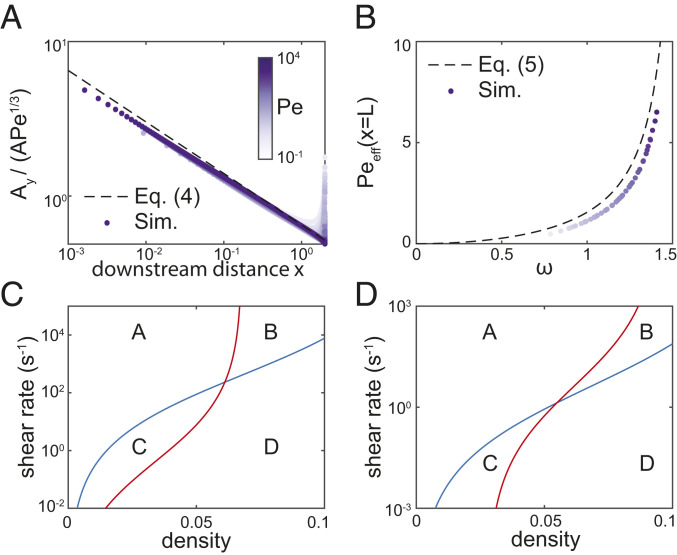
Fig. 2.

An algebraic relationship links flow, biomass, and kinetics at the onset of QS activation. (A) For the simulations in Fig. 1D, when the calculated effective Péclet number at the cell population boundary, $A_y/A$, is scaled by ${\text{Pe}}^{1/3}$, the simulation data collapse onto the curve $0.65/x^{1/3}$ (dashed line), as predicted in Eq. 6 with $D=1$ (both axes scaled logarithmically). Here $A$ is the AI concentration, $A_y$ is its derivative in the vertical direction (perpendicular to the flow), $x$ is the coordinate parallel to the flow, and $y$ is the coordinate perpendicular to the flow. (B) When plotted against the appropriate nondimensional variables identified in Eqs. 6 and 8, the simulations from Fig. 1D collapse onto the curve defined by Eq. 7 (see also SI Appendix, Fig. S4). (C and D) Illustrative examples of how cells can measure density and flow by measuring activation (Eq. 7) of two different AIs, splitting parameter space into four regions A, B, C, and D (vertical axes scaled logarithmically). (C) Cell population of height 10 $\mathrm{\mu }$m. The first AI has kinetic parameters from SI Appendix, Table S1 (blue line), and the second AI also has a factor of 10 reduction in diffusivity in the cell layer and factor of 5 reduction in LuxR production rate (red line) compared to the first AI. (D) Cell population of height 100 $\mathrm{\mu }$m. The first AI has kinetic parameters from SI Appendix, Table S1, but with factor of 10 increase in LuxI and LuxR decay rates (blue line), and the second AI also has a factor of 500 increase in AI decay rate and factor of 2 increase in LuxR production rate (red line) compared to the first AI.