. 2021 Feb 5;10:e63704. doi: 10.7554/eLife.63704

Figure 4. Quantifying the impact of quarantine for returning travellers.

(A) The fraction of local transmission that is prevented by quarantining an infected traveller returning from a 7-day trip. Quarantine begins upon return at time t_Q=0, and we assume that exposure could have occurred at any time during the trip, that is, -7t_E0. Under the standard quarantine protocol (black), individuals are released without being tested [Equation (9)]. The test-and-release protocol (colours) requires a negative test result before early release, otherwise individuals remain isolated until they are no longer infectious (day 10). Colour intensity represents the delay between test and release (from 0 to 3 days). While extended quarantine can prevent 100% of local transmission (grey line), this represents 73.3% [CI: 65.7%,80.3%] of the total transmission potential (see Figure 4—figure supplement 1A). The remaining transmission occurred before arrival. (B) The relative utility of the quarantine scenarios in A compared to the standard protocol 10-day quarantine [Equation 6]. Utility is defined as the local fraction of transmission that is prevented per day spent in quarantine. The grey line represents equal utilities (relative utility of 1). We assume that the fraction of individuals in quarantine that are infected is 10%, and that there are no false-positive test results. Error bars reflect the uncertainty in the generation time distribution.

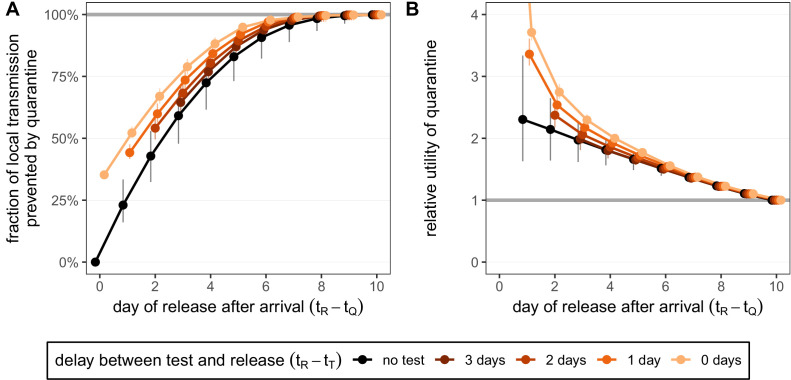
Figure 4—source data 1. Fraction of transmission prevented by quarantine (travellers; local; test-and-release).
Figure 4—source data 2. Relative utility of quarantine (travellers; local; test-and-release).

Figure 4.

Figure 4—figure supplement 1. Quantifying the effect of travel duration and quarantine duration for the standard quarantine protocol (no test) for returning travellers.

Figure 4—figure supplement 1.

(A) The fraction of total transmission that is prevented by quarantining an infected traveller [Equation (7)]. (B) The relative utility of the different quarantine durations in A compared to release on day 10, based on the total fraction of transmission prevented. (C) The fraction of local transmission that is prevented by quarantining an infected traveller [Equation (9)]. (D) The relative utility of the different quarantine durations in C compared to release on day 10, based on the local fraction of transmission prevented. Colours represent the duration of travel y, and we assume that infection can occur with equal probability on each day t_E which satisfies -yt_E0. Quarantine begins at time t_Q=0, which is the time of arrival. Error bars reflect the uncertainty in the generation time distribution.
Figure 4—figure supplement 1—source data 1. Fraction of transmission prevented by quarantine (travellers; total; no test).
Figure 4—figure supplement 1—source data 2. Relative utility of quarantine (travellers; total; no test).
Figure 4—figure supplement 1—source data 3. Fraction of transmission prevented by quarantine (travellers; local; no test).
Figure 4—figure supplement 1—source data 4. Relative utility of quarantine (travellers; local; no test).
Figure 4—figure supplement 2. Quantifying the impact of quarantine and reinforced hygiene measures for returning travellers.

Figure 4—figure supplement 2.

(A) The fraction of local transmission that is prevented by quarantining an infected traveller and enforcing strict hygiene measures after release (see 'Appendix 1: Reinforced prevention measures after early release' for details). The scenarios are the same as in Figure 4 (i.e. exposure occurs with equal probability between day –7 and return at day 0, -yt_E0, and quarantine starts at time t_Q=0), but we reduce post-quarantine transmission by r=50% until day 10, after which further transmission is unlikely. (B) The relative utility of the quarantine and hygiene scenarios in A compared to the standard protocol 10-day quarantine [Equation 6]. We assume that the fraction of individuals in quarantine that are infected is 10%, and that there are no false-positive test results. Error bars reflect the uncertainty in the generation time distribution.
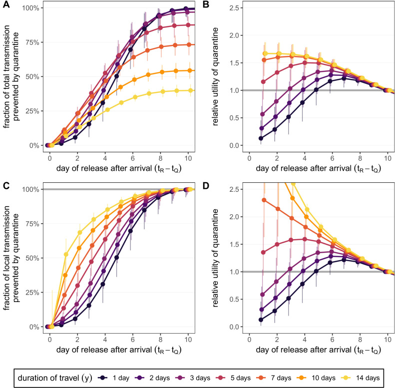
Figure 4—figure supplement 2—source data 1. Fraction of transmission prevented by quarantine (travellers; local; reinforced hygiene).
Figure 4—figure supplement 2—source data 2. Relative utility of quarantine (travellers; local; reinforced hygiene).
Figure 4—figure supplement 3. How adherence and symptoms affect quarantine efficacy for returning travellers.

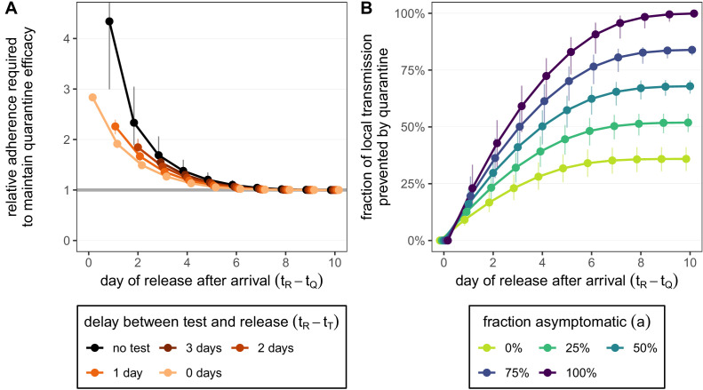
Figure 4—figure supplement 3.

(A) The fold-change in adherence to a new quarantine strategy that is required to maintain efficacy (local fraction of transmission prevented) of the baseline 10-day standard strategy. Quarantine strategies are the same as in Figure 4 (standard = black, test-and-release = colours). The grey line represents equal adherence (relative adherence of 1). (B) The impact of symptomatic cases on the fraction of local transmission per infected traveller that is prevented by standard (no test) quarantine [Equation (A9)]. We assume that symptomatic individuals will immediately self-isolate at symptom onset. The time of symptom onset is determined by the incubation period distribution (see Figure 1—figure supplement 1D). The curve for a=100% corresponds to the black curve in Figure 4A. For both panels, as in Figure 4, we fix the trip duration to 7 days and assume exposure can occur at any time -yt_E0. Quarantine begins at time t_Q=0. Error bars reflect the uncertainty in the generation time distribution.
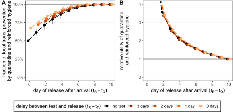
Figure 4—figure supplement 3—source data 1. Relative adherence (travellers; local; test-and-release).
Figure 4—figure supplement 3—source data 2. Role of asymptomatic cases (travellers; local).