Sharpening ECOSTRESS and VIIRS land surface temperature using harmonized Landsat-Sentinel surface reflectances

Abstract

Land surface temperature (LST) is a key diagnostic indicator of agricultural water use and crop stress. LST data retrieved from thermal infrared (TIR) band imagery, however, tend to have a coarser spatial resolution (e.g., 100 m for Landsat 8) than surface reflectance (SR) data collected from shortwave bands on the same instrument (e.g., 30 m for Landsat). Spatial sharpening of LST data using the higher resolution multi-band SR data provides an important path for improved agricultural monitoring at sub-field scales. A previously developed Data Mining Sharpener (DMS) approach has shown great potential in the sharpening of Landsat LST using Landsat SR data co-collected over various landscapes. This work evaluates DMS performance for sharpening ECOsystem Spaceborne Thermal Radiometer Experiment on Space Station (ECOSTRESS) LST (~70 m native resolution) and Visible Infrared Imaging Radiometer Suite (VIIRS) LST (375 m) data using Harmonized Landsat and Sentinel-2 (HLS) SR data, providing the basis for generating 30-m LST data at a higher temporal frequency than afforded by Landsat alone. To account for the misalignment between ECOSTRESS/VIIRS and Landsat/HLS caused by errors in registration and orthorectification, we propose a modified version of the DMS approach that employs a relaxed box size for energy conservation (EC). Sharpening experiments were conducted over three study sites in California, and results were evaluated visually and quantitatively against LST data from unmanned aerial vehicles (UAV) flights and from Landsat 8. Over the three sites, the modified DMS technique showed improved sharpening accuracy over the standard DMS for both ECOSTRESS and VIIRS, suggesting the effectiveness of relaxing EC box in relieving misalignment-induced errors. To achieve reasonable accuracy while minimizing loss of spatial detail due to the EC box size increase, an optimal EC box size of 180–270 m was identified for ECOSTRESS and about 780 m for VIIRS data based on experiments from the three sites. Results from this work will facilitate the development of a prototype system that generates high spatiotemporal resolution LST products for improved agricultural water use monitoring by synthesizing multi-source remote sensing data.

1. Introduction

Thermal satellite data have been widely used for ecological and hydrological studies from local to global scales (Kustas and Anderson, 2009). Land surface temperature (LST) estimated from thermal infrared (TIR) remote sensing imagery, a key parameter in energy balance modeling at the land-atmosphere interface, has been used for a variety of environmental applications, including surface energy flux mapping (Anderson et al., 2008; Anderson et al., 2007; Anderson et al., 2004b; Kustas et al., 2004; Kustas et al., 2003; Norman et al., 2003), evapotranspiration (ET) and soil moisture estimation (Allen et al., 2011; Allen et al., 2007; Anderson et al., 2012; Torres-Rua et al., 2016; Trezza et al., 2008; Yang et al., 2017b; Yang et al., 2018). Accurate estimation of LST is vital to understanding various environmental processes that are facilitated by frequent LST observations with fine spatial resolution. For instance, sub-field-scale ET retrievals at 30-m resolution in near-daily repetition have proven valuable in routine monitoring of agricultural water use and vegetation stress (Anderson et al., 2018; Anderson et al., 2012; Knipper et al., 2019; Sun et al., 2017).

The spatial resolution of TIR bands from thermal sensors tends to be coarser than the surface reflectance (SR) data including visible, near-infrared and shortwave infrared (VSWIR) bands from shortwave sensors on the same platform. Sharpening thermal data to a higher spatial resolution by taking advantage of SR data provides a useful and effective way to add spatial detail to the LST information and data products derived from LST. In the case of ET mapping, thermal sharpening serves to better confine higher evaporative fluxes within crop field boundaries, improving estimates of field-scale water use.

Numerous thermal sharpening approaches have been developed in recent years. One class of sharpening algorithms takes advantage of the empirical relationship between vegetation indices (e.g., Normalized Difference Vegetation Index (NDVI)) and LST through traditional linear or nonlinear regression techniques, such as the TsHARP algorithm proposed by Kustas et al. (2003) and further refined by using fractional vegetation cover rather than NDVI to sharpen LST (Agam et al., 2007b). The two approaches have been widely used in a number of studies (Agam et al., 2007a, 2008; Anderson et al., 2004b; Cammalleri et al., 2008). Besides vegetation, other factors (e.g., land cover type, soil moisture and topography) also play a role in impacting the spatial pattern of LST, motivating a large number of studies that tried to improve thermal sharpening accuracy by integrating indices including land-use data (Bonafoni, 2016; Lillo et al., 2018; Nichol, 2009; Yang et al., 2017c), photosynthetically active vegetation cover (Liu et al., 2018; Merlin et al., 2010), emissivity (Inamdar and French, 2009; Inamdar et al., 2008; Jeganathan et al., 2011), digital elevation model (DEM) data (Hutengs and Vohland, 2016), and albedo (Dominguez et al., 2011) into the sharpening process. These studies suggest that the incorporation of predictors besides NDVI and vegetation cover has the potential to improve the sharpening accuracy over complex landscapes.

The aforementioned sharpening methods are conceptually similar; that is, building empirical relationships between LST and predictors coming from one or a combination of indices (e.g., NDVI) generated from spectral bands or biophysical parameters (e.g., emissivity and albedo). These techniques require adjustment of the predictor variables to obtain optimal sharpening results over different landscapes, inhibiting the flexibility of their use for global applications. To extend the validity domain of thermal sharpening approaches, a number of statistical and machine learning tools have recently been adopted to characterize the regression relationship between LST and SR data, including kriging (Mukherjee et al., 2015; Pereira et al., 2018), random forest (Hutengs and Vohland, 2016; Lillo et al., 2018; Yang et al., 2017c), neural network (Bindhu et al., 2013) and support vector machines (SVM) (Kaheil et al., 2008; Liu et al., 2018). Among them, Gao et al. (2012) developed a Data Mining Sharpener (DMS) based on a multivariate regression tree method (cubist), which has shown its effectiveness in sharpening of Landsat LST and been widely used in many applications (Anderson et al., 2018; Yang et al., 2018). DMS is a data-driven approach that sharpens the TIR data by establishing multivariate regressions that directly utilize reflectance data from all available shortwave bands. DMS shows improved performance over the NDVI-based TsHARP algorithm for Landsat LST sharpening (Gao et al., 2012). In addition, DMS does not require any pre-defined relationship and other higher-order products or parameters (e.g., NDVI) as inputs, allowing flexibility for integration into an operational data production system.

DMS and most other sharpening approaches have typically been tested using thermal and SR data or derived higher-order products collected from the same satellite platform, thereby increasing the spatial resolution but not the temporal resolution of the LST data. In contrast, thermal sharpening involving multi-source data can produce LST data with higher combined temporal frequency, allowing improved monitoring of rapidly changing surface conditions.

For instance, medium-resolution sensors such as the Landsat 8 Operational Land Imager (OLI) and Thermal Infrared Sensor (TIRS) package (Roy et al., 2014) provide both VSWIR and TIR images at spatial resolutions of 30 m and 100 m, respectively (Table 1). Thermal sharpening of Landsat LST to 30 m using Landsat SR data has been used in many studies to improve the spatial resolution of evapotranspiration (ET) mapping (Anderson et al., 2012). However, the temporal frequency of Landsat image acquisition (16 days with a single platform) can be limiting for robust ET monitoring, particularly in regions of persistent cloud cover (Yang et al., 2017a). The Sentinel-2a and −2b satellites provide SR data at 10–20 m spatial resolution and 10-day (or 5-day combined) revisit period; however, Sentinel-2 does not collect TIR data (Table 1). The Harmonized Landsat and Sentinel-2 (HLS) dataset provides a unified collection of SR data acquired by Landsat 8 and Sentinel-2 and provided as three products: S10 (Sentinel-2 10 m), S30 (Sentinel-2 30 m) and L30 (Landsat-8 30 m) (Claverie et al., 2018). The high temporal resolution of HLS makes it attractive for thermal sharpening on LST data from other satellite platforms. For example, NASA’s recently launched ECOsystem Spaceborne Thermal Radiometer Experiment on Space Station (ECOSTRESS) provides TIR bands with around 70-m spatial resolution and an average of 4-day revisit frequency (Table 1) but does not collect VSWIR data (Fisher et al., 2015; Hulley et al., 2017). The Visible Infrared Imaging Radiometer Suite (VIIRS) that was launched in 2011 provides TIR data at 375-m resolution (I5 band) on a near-daily basis. The availability of these additional TIR data sources, along with the HLS SR dataset, holds a great potential to generate 30-m LST products with high combined temporal frequency.

Table 1.

Spatial and temporal resolutions of different satellite data sources for SR and TIR bands.

Platform/sensor	SR bands	TIR bands	Revisit	Availability
Landsat 8	30 m	100 m	16 day	2013+
Sentinel-2A	10–20 m		10 day	2015+
Sentinel-2B	10–20 m		10 day	2017+
HLS (S30)	30 m		3–4 day	2015+
ECOSTRESS		~70 m	< 4 day	2018+
VIIRS I bands	375 m	375 m	~daily	2011+

Thermal sharpening using multi-source data can present new challenges resulting from sensor differences in geo-referencing, acquisition date/time and data quality. Few studies have investigated the performance of thermal sharpening utilizing multi-platform data and the impact from the mentioned difficulties (Bisquert et al., 2016; Cammalleri et al., 2008; Guzinski and Nieto, 2019; Pereira et al., 2018). While the DMS has shown good skill for sharpening using Landsat platform data (Gao et al., 2012), its utility for thermal sharpening based on data from multi-platforms remains unclear. Recently, a Python implementation of DMS (pyDMS) has been released by Guzinski and Nieto (2019) in Github, widely increasing its exposure to the community for a wide range of applications including multi-sensor ET mapping using Sentinel-2 and 3 data. However, issues that may exist in the application of DMS to muti-platform data may be mishandled by less experienced users. Improved understanding of the DMS performance for multi-platform data is urgently needed to expand utility in operational applications.

In this study, we evaluate the capability of the DMS approach for thermal sharpening across platforms and explore ways to reduce the impacts of differences in TIR-SR geolocation accuracy. Thermal data from ECOSTRESS and VIIRS over target sites in California were sharpened to 30-m resolution using HLS SR data and compared to reference images from Landsat 8 and unmanned aerial vehicle (UAV) acquisitions. First, typical ECOSTRESS/VIIRS TIR misalignments with respect to the SR data are quantified, and then a modified DMS is proposed to relieve the influence of these misalignments. We also investigate the impact on sharpening performance of different methods for resampling the swath TIR data provided by ECOSTRESS and VIIRS to the SR grid, which has been shown to affect sharpening results (Allen et al., 2008; Chen et al., 2014; Singh Rawat et al., 2019; Sismanidis et al., 2017).

Section 2 gives a brief description of the standard DMS algorithm and the proposed modified version. Section 3 describes the study area and data preparation. The results and discussion are provided in Sections 4 and 5, respectively, followed by the conclusions in Section 6.

2. Modeling approach

2.1. Data Mining Sharpener (DMS)

The Data Mining Sharpener (DMS) algorithm proposed by Gao et al. (2012) is implemented via the following four steps. First, the SR images are aggregated to the native TIR spatial resolution and a sample of relatively homogeneous pixels are selected from the coarse-resolution SR and TIR images. Homogeneity is defined based on the sub-pixel coefficient of variation (CV) in the SR data, which is expressed as follows:

$$c_v=\left(1/n\right){\sum }_{i=1}^n\left({\sigma }_i/{\mu }_i\right)$$

where n is the total number of spectral bands, and μ_i and σ_i represent the mean and standard deviation of the fine spatial resolution pixels within each coarse resolution pixel in band i. We use the threshold c_v < 0.1 to select coarse-resolution samples for Landsat and ECOSTRESS LST sharpening, while a larger threshold, c_v < 0.2, is used for VIIRS due to the coarser native pixel size. Second, the homogenous SR and TIR samples at coarse resolution are used to train and build a cubist regression tree. Next, this regression tree is applied to the SR images at their native resolution to estimate LST at fine pixel resolution. The final step aggregates the sharpened LST at fine resolution to the TIR band resolution and computes the differences (residuals) from the raw LST map at its original coarse resolution. The residuals are redistributed over the fine-scale LST map, either uniformly or smoothly using bilinear interpolation. This step is aimed at enforcing energy conservation (EC) within the sharpening process. For brevity, we call this step EC.

Gao et al. (2012) used two models - a global and a local model - to select samples for regression tree training. The global model trains a regression tree for sharpening using samples selected from the entire image. The local model trains the local regression tree using samples within a local moving window. Each local window overlaps with surrounding windows to avoid artificial effects at the window boundary. The local model tends to have overall better performance than the global model (Chen et al., 2012; Gao et al., 2012; Jeganathan et al., 2011; Zakšek and Oštir, 2012). However, the local model may have lower prediction accuracy for some outlier features that are not well represented within the smaller moving window. Thus a combined model, taking advantage of both global and local modeling approaches, was proposed (Gao et al., 2012). It should be noted that the local model demands more computing time than the global model and results depend on the complexity of the area and moving window size. For simplicity and a more consistent comparison across data sources, this paper only uses the global modeling approach. More details can be found in Gao et al. (2012).

The cubist regression tree method has an optional boosting-like procedure called committees that determine the number of iterative model trees that are created in sequence. A new model tree is created using adjusted training set outcomes from the last tree. The final model prediction is the average of each model tree prediction. While the committee approach increases computing time, we found it was helpful in eliminating some anomalous behavior (see the specified area in Fig. 1a for example). Therefore, in this study, we use five committees for ECOSTRESS and VIIRS LST sharpening which produced improved results (Fig. 1b).

Fig. 1.

Sharpened images (central point: 121°6′W, 38°17′N) of ECOSTRESS LST (°C) with 180-m EC size and (a) one or (b) five committees; (c) the NIR-red-green composite of Landsat 8 SR data. The anomalous feature highlighted in (a) is removed through the use of five committees in (b).

2.2. Modifications to the DMS approach

The DMS algorithm has been successfully applied in thermal sharpening using TIR and SR data from the same sensor, collected at the same time and well co-registered. As previously discussed, LST and SR data from different sensors might not be geometrically consistent in terms of precise registration and orthorectification, leading to some degree of mismatch between the two datasets. An example is shown in Fig. 2 in which we use the standard DMS algorithm to sharpen both Landsat 8 and ECOSTRESS LST using Landsat 8 SR data. It is clearly seen that, for many locations, the sharpened ECOSTRESS LST shows significantly blurrier boundaries than the sharpened Landsat 8 LST. These “shift artifacts” are attributed in part to the image misalignment between Landsat 8 and ECOSTRESS.

Fig. 2.

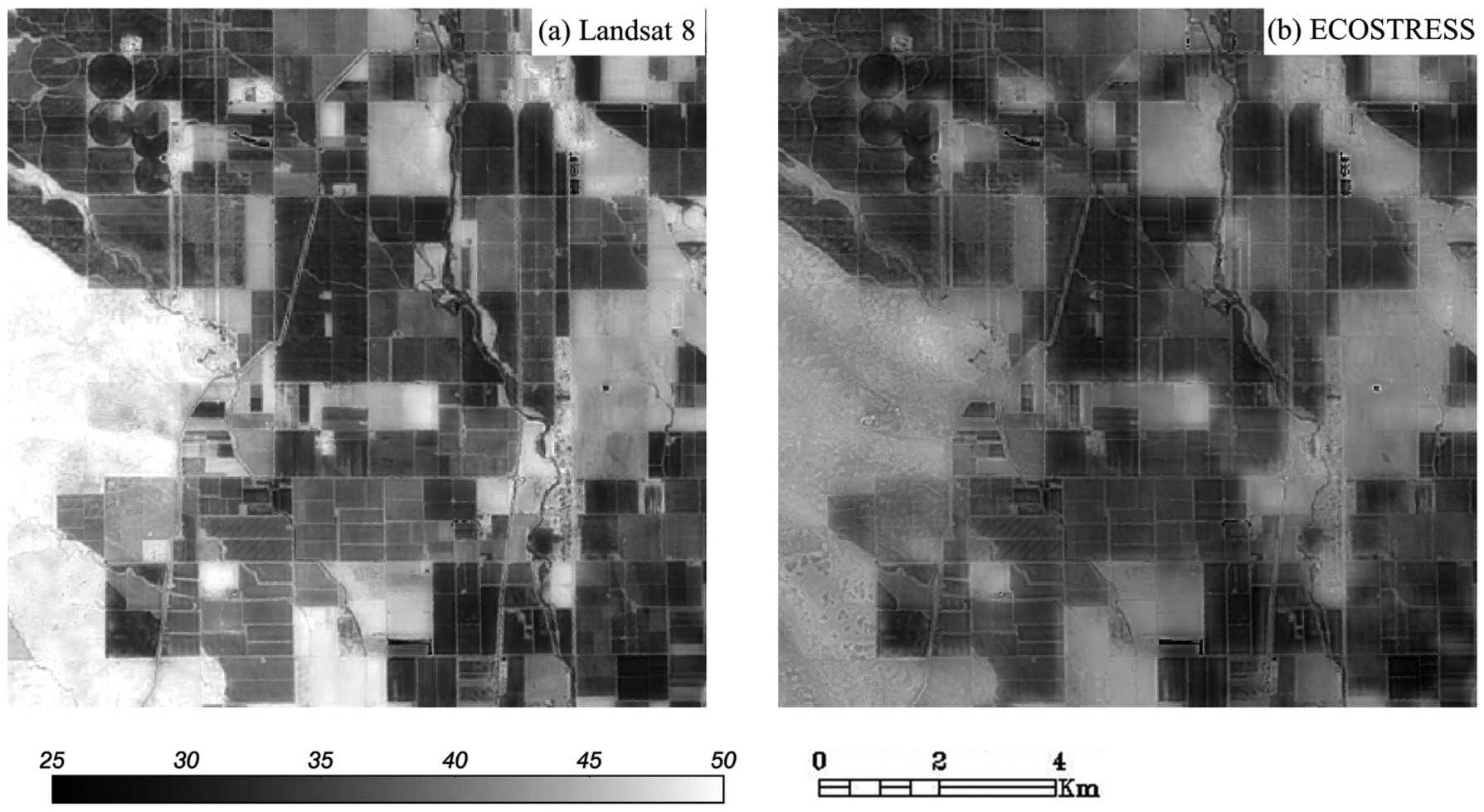
Sharpening results (central point: 122°14′W, 39°38′N) of LST (°C) at 30 m resolution using the standard DMS algorithm for (a) Landsat 8 and (b) ECOSTRESS. Both used the same Landsat 8 SR to sharpen the LST images. The mismatch (shift) between ECOSTRESS and Landsat caused blurring effects after applying the energy conservation process using a 90-m EC box in (b).

In the standard DMS approach, a homogeneous pixel at coarse resolution is determined based on the sub-pixel CV using fine resolution pixels within the coarse cell. For Landsat 8 LST sharpening, 3 × 3 30 m resolution SR pixels were used to determine a homogeneous LST pixel (100 m resolution). In the modified version, a homogeneous pixel is computed using an extended area (± 1 pixel) to reduce the effect of misalignment. For example, ECOSTRESS and VIIRS LST sharpening uses 5 × 5 and 15 × 15 30 m resolution pixels to determine a homogeneous LST pixel and then averages the central 3 × 3 and 13 × 13 pixels to generate LST-SR samples, respectively. The stricter rule ensures that only large homogeneous pixels are used in building regression trees. The extended sampling window is expected to help reduce the co-registration errors.

The EC process in the standard DMS approach conserves energy at the native thermal band pixel scale, maximizing the propagation of spatial TIR information into the sharpened image. In this paper, we propose to use a relaxed EC box size, that is, to aggregate both the original and sharpened fine-resolution LST to a resolution coarser than the nominal native TIR resolution before computing the residuals. The relaxing of EC box size is expected to help relieve the co-registration errors or the shift effect by increasing the area of overlap between the TIR and SR information within the EC box. For co-registration differences (shifts) ranging from 30 m to 150 m, the change of the overlapped area with respect to EC box size is shown in Fig. 3. For example, given a relative shift of 30 m (in both dimensions) between TIR and SR data layers, an EC box of 90 m will contain 44% overlap of consistent area, while an EC box of 180 m or 270 m will provide 69% or 79% overlapped area respectively as highlighted in Fig. 4. The use of a larger EC box size results in a larger overlapped area, which is expected to provide a greater relief from the co-registration errors. However, the increase of EC box size may also lead to spatial thermal information loss in the sharpened image. In addition, the value added by increasing the EC box size begins to asymptote at some level, as highlighted in Fig. 3. Consequently, an appropriate EC box size will balance the need to accommodate misregistration while preserving thermal information content in the sharpened image. This paper aims to explore the response of sharpening accuracy to EC box size, which will provide insights on determining an optimal EC box size for different sensors with different geolocation accuracies. The DMS approach has been revised to take the EC box size as an input variable.

Fig. 3.

The percentage of the overlapped area (y-axis) of TIR and SR information within an EC box with respect to relative geolocation error (shift) and EC box size (x-axis).

Fig. 4.

A schematic illustrating the area of overlapping SR and TIR information content with respect to EC box size from 90 m to 270 m for a 30-m TIR image shift in both dimensions.

3. Data and analyses

3.1. Study area and datasets

The standard and modified DMS approaches were tested over domains including three study sites within California, USA, that are part of the USDA-ARS Grape Remote Sensing Atmospheric Profile and Evapotranspiration eXperiment (GRAPEX) (Kustas et al., 2018). As illustrated in Fig. 5, the three GRAPEX sites are Sierra Loma vineyard near Lodi, California in Sacramento County, Barrelli vineyard near Cloverdale, California, and Ripperdan vineyard near Madera, California. The land cover types in three areas are mainly irrigated vineyards surrounded by irrigated orchards, unirrigated pastures and grasslands, and in combination they sample a significant north-south climate and vegetation gradient due to variations in temperature, vapor pressure and precipitation.

Fig. 5.

Sierra Loma, Barrelli and Ripperdan sites in California, USA.

To facilitate intercomparison, for each site we identified dates with same-day overpasses of Landsat 8, ECOSTRESS and VIIRS, with a focus on the period of available ECOSTRESS imagery in 2018 (August–September). Given prior demonstrated utility of DMS with Landsat data (Anderson et al., 2018; Knipper et al., 2019), sharpened 30-m Landsat 8 LST images, where available, serve as the baseline for evaluating DMS performance with ECOSTRESS and VIIRS. Landsat sharpening represents a best-case scenario, where both TIR and SR data are collected simultaneously from the same platform and are well co-registered, and the sharpening ratio (factor of 3) is relatively small. The Sierra Loma and Barrelli sites had same-day overpasses on 04 August and 11 August 2018, respectively (Table 2). However, at Ripperdan only Landsat 7 was available for dates with same-day overpasses of ECOSTRESS and VIIRS in 2018. In that case, we used Sentinel-2 SR data for sharpening to avoid scan-line corrector gap issues in Landsat 7. At this site, very high-resolution imagery collected via unmanned aerial vehicles (UAVs) from the Utah State University AggieAir UAV Research Group (https://uwrl.usu.edu/aggieair/) is available for 05 August 2018 when good-quality ECOSTRESS and VIIRS LST data are also available, providing an opportunity to evaluate thermally sharpened images directly at the 30-m scale.

Table 2.

Three study sites and the corresponding SR and TIR data used in the sharpening experiments.

Test site	Date (DOY)	SR data	Resolution (m)	TIR data	Resolution (m)	Time (PST)	View angle
Sierra Loma	08/04/2018 (216)	Landsat 8 (p44r33)	30	Landsat 8	100	10:45 am	<7°
				ECOSTRESS	~70	2:54 pm	16.5°
				VIIRS	375	1:30 pm	40.3°
Barrelli	08/11/2018 (223)	Landsat 8 (p45033)	30	Landsat 8	100	10:51 am	< 7°
				ECOSTRESS	~70	12:04 pm	16.8°
				VIIRS	375	1:30 pm	16.7°
Ripperdan	08/05/2018 (217)	Sentinel-2 (S30, T11SKA)	30	UAV	0.6	12:34 pm	< 7°
				ECOSTRESS	~70	2:03 pm	16.3°
				VIIRS	375	1:30 pm	17.9°

Calibrated and atmospherically corrected Landsat 8 SR products were downloaded from the U.S. Geological Survey (USGS) Earth Explorer (http://earthexplorer.usgs.gov/) for the Sierra Loma and Barrelli sites (WRS-2 path 44 and row 33, and path 45 and row 33, respectively). These SR data were used to sharpen Landsat, ECOSTRESS and VIIRS TIR data on the same-day overpass dates. For the Ripperdan site, Sentinel-2 SR data, S30 (Tile 11SKA) product from the NASA Harmonized Landsat Sentinel-2 (HLS) project (http://hls.gsfc.nasa.gov/), were used instead to sharpen ECOSTRESS and VIIRS LST. Landsat 8 at-sensor brightness temperature observations (resampled to 30-m resolution using the cubic convolution method) downloaded from USGS were atmospherically corrected via MODTRAN (Berk et al., 1987) following procedures developed for the Landsat Collection 2 standard LST product (Cook et al., 2014) and using input atmospheric profiles from the Modern-Era Retrospective analysis for Research and Applications, Version 2 (MERRA-2; Rienecker et al., 2011). ECOSTRESS Level 2 Land Surface Temperature and Emissivity products collected from Jet Propulsion Laboratory are atmospherically corrected with the Radiative Transfer for TOVS algorithm (RTTOVS; Saunders et al., 2018) with atmospheric profiles from the Goddard Earth Observing System Model, Version 5 (GEOS-5) reanalysis product (Bosilovich et al., 2008). VIIRS I5 at-sensor brightness temperature observations (resampled to a 0.004 degree resolution using bilinear interpolation) were downloaded from NASA LANCE and atmospherically corrected using a single channel inversion (Price, 1983) based on atmospheric profiles of temperature and moisture from the Climate Forecast System Reanalysis V2 (Saha et al., 2014). Radiometrically and geometrically calibrated ECOSTRESS LST and VIIRS TIR swath data products over the three sites were gridded to the same spatial grid (30 m, UTM projection) as the Landsat 8/HLS (S30) SR data prior to sharpening to avoid artificial pixel misalignments when cutting them to the same size. Tests regarding swath gridding methods are described in Section 3.2 with results shown in Section 4.4.1. During the sharpening process, the resampled 30-m LST was first aggregated to approximately native resolution for training LST-SR relationship, to 90 m for Landsat and ECOSTRESS and 390 m for VIIRS.

UAV LST over the Ripperdan site was collected from flights performed at an elevation 400 m (~1300 ft) above ground level and completed within 20 mins to ensure the changes of surface temperature in time is less than 0.5 K (restriction is based on patterns found from ground temperature measurements). The on-board instrumentation includes the custom 12MP Red-Green-Blue and NIR optical sensors, and a radiometrically calibrated thermal camera (model 9640-P) from Infrared Cameras Incorporated (ICI; https://infraredcameras.com/), which were integrated into a UAV payload by the AggieAir UAV Research Group. Thermal images were processed using Agisoft software (https://www.agisoft.com/downloads/user-manuals/) under the Average Blending mode during Texture generation. The resulted thermal image and emissivity were not corrected for atmospheric effects due to the lack of local emissivity values for vineyards and soil, while estimation of emissivity for thermal sensors at a small pixel scale (submeter) remains an active area of research (Torres-Rua et al., 2019; Torres-Rua et al., 2020).

For the Sierra Loma and Barrelli sites, sharpened ECOSTRESS and VIIRS LST were compared to sharpened Landsat 8 LST data. For Ripperdan, UAV data on 5 August were collected at both 10:44 AM (typical Landsat time) and 12:34 PM (solar noon); the latter with an acerage of ~1 mile² was selected for comparison, being closer to the ECOSTRESS and VIIRS overpass times (Torres-Rua et al., 2018). The UAV LST data were also projected to the same projection system and resampled to 30 m resolution to facilitate the comparison with sharpened results. All the SR and TIR data used in sharpening tests and the corresponding acquisition date, overpass time, view angle and nominal resolution are summarized in Table 2. While Landsat scenes are constrained to view angles of < 7°, the ECOSTRESS and VIIRS swaths extend to ~25° and ~56°, respectively, with potential impacts on effective resolution and sharpening performance. Anderson et al. (2020, in review) note degradation in ECOSTRESS resolution beyond ~20°. The sub-swath scenes used here, however, were all collected at view angles < 17° and do not show significant visual impacts of resolution degradation. Compared to VIIRS predecessors, an important design feature of VIIRS is constrained off-nadir pixel growth (Cao et al., 2013; Schueler et al., 2013; Wolfe et al., 2013). Specifically, VIIRS restricts the pixel to at most two-fold (2:1) growth from nadir to edge-of-scan (~56° off-nadir). Although the view angle on DOY 216 over Sierra Loma site is relatively large (40°) and there is some degradation of VIIRS pixel size (up to ~600 m), the use of a relaxed EC box size in our thermal sharpening is expected to relieve the impact of this issue.

Prior to sharpening, pixels contaminated by forest fires and smoke plumes, clouds and cloud shadows at all sites were excluded using the QA band generated from the CFMask algorithm (Zhu and Woodcock, 2012) for Landsat/HLS-S30, L2 Cloud mask for ECOSTRESS, and the cloud mask associated with the fire product (375-m I-band) for VIIRS. Within the Barrelli domain, ocean pixels were additionally masked out, leading to a greatly reduced number of pixels for sharpening. Therefore, the threshold c_v is set as 0.15 for Landsat and ECOSTRESS and 0.25 for VIIRS LST sharpening respectively over the Barrelli domain. With these thresholds we obtain approximately 252,254 (36.5% of all pixels) and 14,491 (40.3%) samples for training cubist regression trees for Landsat/ECOSTRESS LST sharpening and VIIRS LST sharpening, respectively. Similarly, we obtain 723,267–1,284,785 (37.8%–50.2%) samples for Landsat/ECOSTRESS sharpening and 35,671–79,656 (47.8%–50.8%) samples for VIIRS sharpening over the Sierra Loma and Ripperdan domain. For both Landsat 8 and HLS (S30), SR data from six VSWIR bands (Blue, Green, Red, NIR (B8A for S30), SWIR 1 and SWIR 2) bands were employed to sharpen TIR LST data. Surface reflectance has been shown to aggregate linearly by simple areal averaging (Anderson et al., 2004a), while TIR data are more appropriately aggregated according to the fourth power of Stephan–Boltzmann law (Agam et al., 2007b). For LST aggregation, LST was first converted to radiance following Stephan–Boltzmann law, the radiances were averaged to the target coarse resolution and then converted back to temperature fields. Linear aggregation of LST without considering the Stephan-Boltzmann law was also employed in previous studies (Merlin et al., 2010) and only small differences were obtained between the two aggregations (Liu et al., 2006). In DMS sharpening, we employed the Stephan–Boltzmann law for LST aggregation.

3.2. Swath TIR data gridding methods

ECOSTRESS L2 LST and VIIRS 375 m TIR data are both provided in swath format and need to be gridded and resampled to the SR grid prior to sharpening. Studies have demonstrated that the proper combination of gridding/resampling and sharpening techniques can improve sharpening results (Chen et al., 2014; Singh Rawat et al., 2019; Sismanidis et al., 2017). Allen et al. (2008) suggested the use of the nearest neighbor (NN) method for LST resampling, which allows the identification of locations of the original thermal pixels. However, for thermal sharpening involving multi-sensor data, image co-registration errors between the VSWIR and thermal bands may reduce the reliability of the NN method. Bilinear interpolation is another widely used resampling approach for gridding thermal images to VSWIR image scale for sharpening (Anderson et al., 2004b). This approach may help to relieve geolocation errors induced by image misalignments because it incorporates adjacent pixels for resampling. Given these considerations, we evaluated the feasibility of both NN and bilinear interpolations in resampling VIIRS LST in conjunction with the DMS sharpening approach. The method with the better performance was then selected for further use. VIIRS was used for this test because the scale difference between the native (375 m) and target (30 m) image for VIIRS is much larger than that of ECOSTRESS. The difference in resampling strategies therefore has a larger impact on gridding and sharpening results for VIIRS LST than for ECOSTRESS LST.

3.3. Experiment design

The primary goal of this study is to examine the utility of the standard and modified DMS algorithm for thermal sharpening based on multi-source data and to identify optimal EC box sizes for operational applications. To achieve this goal, we conducted a series of registration and sharpening experiments.

We first quantified misregistration errors for the selected ECOSTRESS and VIIRS LST scenes relative to the Landsat 8/HLS (S30) SR data. We employed five spatial subsets for each study site that include a variety of landscape structures and vegetation cover classes to have a good representation of land types. For each subset, the LST grid was shifted N-S and E-W in 30-m increments over a range of ± 5 and 13 pixels for ECOSTRESS and VIIRS, respectively. For each shift, we computed the correlation coefficient (CC) between LST and NDVI computed from the red and NIR SR data. The magnitude of the shift vector associated with the maximum CC was defined as the nominal image misalignment.

In the next step, we conducted two types of simulated sharpening experiments, emulating idealized ECOSTRESS and VIIRS sharpening, by using SR and LST data from Landsat 8. In the simulated-ECOSTRESS case, the Landsat 8 LST at native resolution (comparable to ECOSTRESS native resolution) were shifted relative to the SR images in varying magnitudes encompassing the typical misalignment identified in the first step. To simulate misalignments between VIIRS LST and Landsat 8 SR images, the Landsat 8 LST images were first resampled to 390 m (comparable to VIIRS native resolution) and then shifted by varying increments. The shifted LST images in both cases were sharpened to 30-m resolution and compared with the 30-m reference LST that was sharpened from the original (unshifted) Landsat LST. The aggregated and shifted Landsat LST data at ~390-m scale (VIIRS simulation) were also sharpened to 90-m resolution and compared with unsharpened Landsat LST for an evaluation at the Landsat native scale. The simulated experiments help us to understand the impact of the image misalignment on sharpening in the absence of other factors (e.g., differences in overpass time and view angle). The experiments were conducted over the Sierra Loma site.

Finally, we conducted actual sharpening experiments over the three target sites (Sierra Loma, Barrelli and Ripperdan), refining ECOSTRESS/VIIRS LST images to 30-m resolution using Landsat/HLS (S30) SR data. In comparison with the simulated sharpening, differences in LST/SR image characteristics (e.g., overpass time and view angle) among sensors and the intrinsic geolocation errors for ECOSTRESS and VIIRS can affect the results. For the Sierra Loma and Barrelli sites, SR data were obtained from Landsat 8 and the sharpened 30-m ECOSTRESS and VIIRS LST were evaluated against sharpened 30-m Landsat 8 LST. In addition, VIIRS LST was also sharpened to 90-m resolution for a direct comparison with the Landsat 8 LST without sharpening (~100 m native resolution). For the Ripperdan site, the HLS S30 product was used to sharpen ECOSTRESS/VIIRS LST due to the lack of Landsat 8 SR data. The aggregated 30-m UAV LST was used as a reference to evaluate the sharpened results at this site.

3.4. Evaluation metrics

Sharpening results from the modified DMS technique were evaluated both visually and quantitatively. An essential motivation of the modified DMS approach with a relaxed EC box size is to help relieve impacts of registration errors on the sharpened image, such as blurriness at boundaries and discontinuities shown in the example in Fig. 2. This both improves the visual fidelity of the sharpened image as well as the spatial correspondence with surface reflectance-based inputs to land-surface modeling systems. Therefore, visual comparisons between sharpened and reference LST imagery play an important role in our evaluation, providing a qualitative understanding of the sharpening accuracy and potential artifacts.

Along with visual comparisons, we rely on the quantitative evaluation to help determine an optimal EC box size that jointly minimizes the impacts of registration errors (reducing blurry boundaries) while maximizing information content (fidelity to the unsharpened image) in the sharpened image. For quantitative evaluation, we used statistical metrics including correlation coefficient (CC) and Nash-Sutcliffe model efficiency coefficient (NSE) (Nash and Sutcliffe, 1970) to assess the spectral similarity between sharpened and reference LST. CC is not sensitive to systematic errors, so it is not heavily impacted by large systematic over- or underprediction. Unlike CC, NSE is sensitive to dispersions of data (Krause et al., 2005; Legates and McCabe Jr, 1999). As complements to CC and NSE, Mean Absolute Error (MAE) and Root Mean Square Error (RMSE) were used to quantify the difference between sharpened and reference LST data, which includes both systematic and unsystematic errors. RMSE is relatively more sensitive to the variability of errors than MAE. RMSE can be divided into Systematic Root Mean Square Error (RMSE_s) and Unsystematic Root Mean Square Error (RMSE_u), as defined in Eq. (1) (Willmott et al., 1985):

$$\text{RMSE=}\sqrt{\frac{1}{N}{{\sum }_{i=1}^N\left(P_i-O_i\right)}^2}$$ (1a)

$${\text{RMSE}}_{\text{s}}\text{=}\sqrt{\frac{1}{N}{{\sum }_{i=1}^N\left(\widehat{P_i}-O_i\right)}^2}$$ (1b)

$${\text{RMSE}}_{\text{u}}\text{=}\sqrt{\frac{1}{N}{{\sum }_{i=1}^N\left(\widehat{P_i}-P_i\right)}^2}$$ (1c)

where P_i and O_i represent sharpened and reference LST value at location i, N is the number of total pixels in the LST image, and ${\widehat{P}}_i$ is the ordinary least square estimate of P_i derived from the regression of P on O. RMSE_s estimates the model’s linear (i.e., systematic) error while RMSE_u evaluates the amount of the discrepancy that comes from randomness or other error sources. Unless the sharpened ECOSTRESS or VIIRS LST images are collected at the same time as the reference LST images (Landsat or UAV), which rarely occurs for cases employing multiple sensor data, the diurnal changes in LST can lead to systematic discrepancies that are real and cannot be corrected for by the sharpening process. For most cases, we rely primarily on CC or RMSE_u, in which the impact from diurnal LST changes can be largely eliminated.

To ensure that the sharpening process does not strongly alter the LST map at its native scale, an additional fidelity metric is also introduced. Fidelity is evaluated by the RMSE between the unsharpened LST map and the sharpened map reaggregated to native resolution. Optimal sharpening parameters will tend to both maximize CC with the reference LST image and minimize the lack of fidelity with respect to the original LST image.

4. Results

4.1. Typical sensor image misalignment

For sharpening involving multi-sensor data, image misalignment between TIR and VSWIR datasets due to differences in geolocation accuracy is a key reason for the use of a relaxed EC box size. To assess expected misregistration errors between ECOSTRESS/VIIRS and Landsat 8/HLS (S30), we evaluated correlations between LST and shifted NDVI over the three study sites for a range of inter-image 30-m shifts. To better sample different landscape structures, we employed five spatial subsets for each study site that include a variety of landscapes and landcover types. Shifts ranged between −5 and 5 pixels in both x and y for ECOSTRESS and − 13 to 13 for VIIRS considering their differences in spatial resolutions. The CC between NDVI and LST was then computed after each shift, and the shift corresponding to the maximum CC was regarded as the optimal shift or nominal image misalignment.

For both ECOSTRESS and VIIRS data over the three sites, it was found that the identified misalignment varied among the different subsets, suggesting spatial heterogeneity in geolocation accuracy difference. Consequently, the optimal shift identified in this study may only represent the ‘average’ misalignment of the entire scene, so we also report the range in identified shifts. The range of the magnitude of the shifts for the ECOSTRESS data is 30–67 m (46 m on average), 0–42 m (26 m), and 42–67 m (54 m), for Sierra Loma, Barrelli and Ripperdan respectively – nominally 30–90 m in terms of integral 30-m Landsat pixel units. For VIIRS data, the magnitude of the shifts over the three sites ranges from 60 to 95 m (75 m), 67–150 m (102 m), and 95–134 m (115 m), respectively – nominally 60–150 m. These expected errors will have ramifications for the selection of sensor-specific EC box size. For reference, the spatial co-registration error between Landsat and Sentinel-2 data is around 15 m for the 30-m products (L30 and S30) of HLS (Claverie et al., 2018). The geolocation accuracy at nadir of ECOSTRESS is on the order of 50 m (Smyth and Leprince, 2018) and that of VIIRS is on the order of 85 m (Cao et al., 2013; Wang et al., 2017; Wolfe et al., 2012).

4.2. Landsat sharpening with simulated shifts

The capability of the standard DMS approach for sharpening Landsat LST to 30 m has been assessed over various land cover types (Gao et al., 2012). The sharpened 30-m LST shows reasonable accuracy and structure and has been widely applied to field-scale ET and crop yield mapping (Anderson et al., 2012; Knipper et al., 2019; Sun et al., 2017). Therefore, this 30-m LST, representing an optimal DMS sharpened result, is used here as a reference in investigating the impact of the relaxed EC box size on sharpening using misaligned images in attempts to reduce artifacts as evident in Fig. 2. Aggregated Landsat LST serves as a proxy for ECOSTRESS and VIIRS thermal imagery with known registration errors.

4.2.1. Simulated ECOSTRESS experiment

In this experiment, the Landsat 8 LST images at native resolution (100 m; close to ECOSTRESS resolution) were artificially shifted with respect to the SR images by 30 to 150 m in the northwest (NW) and southeast (SE) directions. The LST images were then sharpened to 30-m resolution using a set of EC box sizes ranging from 90 m to 1530 m with a 90-m interval, where the 90-m EC box size refers to the standard DMS method. The sharpened results were visually and quantitatively compared with the reference LST (i.e., unshifted Landsat 8 LST sharpened to 30-m). The sharpening results were similar for shifts toward the NW and SE based on quantitative metrics; therefore, only results from the SE shifts are illustrated (Fig. 6).

Fig. 6.

(a) CC, (b) NSE, (c) MAE and (d) RMSE between the sharpened LST (subject to pre-sharpening shifts of 30–150 m) and the reference sharpened Landsat LST as a function of EC box size; (e) RMSE between the sharpened LST reaggregated to 90 m and the unsharpened Landsat LST as a function of EC box size and without EC (labelled as ‘ < no EC > ’).

As shown in Fig. 6, the sharpening test with the smallest image shift results in the highest accuracy and fidelity, highlighting the undermining effect of sensor misalignment on thermal sharpening. For tests with image shifts of 30 and 60 m, the sharpening accuracy shows a declining trend with EC box size, and the highest accuracy is achieved using the smallest EC box size of 90 m, close to the native resolution of the LST imagery. However, this trend changes as the image shift increases to 90 m or larger. In these tests, relaxing the EC box size from 90 to 180 m – as in the modified DMS approach – produced improved sharpening results. This upward trend slows and eventually reverses as EC box size continues to increase, indicating diminishing returns in relieving the shift-induced misregistration. This may be attributed to 1) loss of high spatial frequency LST information as the sharpened image increasingly reflects the SR image content and 2) the fact that the increase of the area of overlapped LST and SR information gradually becomes marginal as seen in the trends shown in Fig. 3. Factor 1 is quantified by the fidelity metric in Fig. 6e. The use of EC boxes with increasing size will generally degrade the fidelity of the sharpened LST image at the native resolution scale, while sharpening without imposing EC process may lead to large errors (Fig. 6e).

In combination, these indicators narrow the selection of an optimal EC box size. Based on the quantitative metrics, the optimal EC box sizes for 90-, 120-, 150-m image shifts are around 270–360 m, 360–540 m, 540–630 m, respectively. Larger misalignment errors require a larger EC box size to obtain the optimal performance. The sharpening simulation tests suggest that the overlapped area should reach around 45–55% (as shown in Fig. 4) to obtain optimal sharpening results.

Fig. 7 demonstrates the impacts of the EC box size relaxation in sharpening an LST image with an artificial shift of (4, −4) pixels/(120, −120) m in the SE direction. Compared to the reference sharpened LST image (Fig. 7b), the misregistered image sharpened using a 90-m EC box has blurry edges and bleeding of structure across sharp field boundaries (Fig. 7c). In contrast, the use of a 270-m EC box substantially reduces these effects (Fig. 7d). Absolute differences between sharpened and reference images show that the 90-m EC box produced large residuals around object edges, while residuals are smaller and more diffused when using a 270-m EC box (Fig. 7g–h).

Fig. 7.

(a) Landsat 30-m NIR-Red-Green composite for the 400 × 400 Sierra Loma study site subset (central point: 121°6′W, 38°16′N) on August 4, 2018; (b) sharpened 30-m Landsat LST (reference; °C); sharpened images of shifted Landsat LST (°C) to SE direction (4,−4) with (c) 90-m EC box size and (d) 270-m EC box size; (e) USGS resampled 30-m Landsat LST (°C); (f) unsharpened 90-m Landsat LST (°C); (g) absolute difference images (°C) between (b) and (c); (h) absolute difference images between (b) and (d). The left greyscale bar is for (b)-(f) while the right bar is for (g)-(h).

It should be noted that, for the simulated experiment, the artificial image shift (co-registration error) is the only factor impacting the performance of the modified DMS approach. In contrast, for real sharpening experiments involving multi-sensor data, other factors including acquisition time differences between sensors also play a role. It is reasonable to hypothesize that the effect of image misalignment in real LST images will be larger than in the simulated experiments. For ECOSTRESS, the 90-m shift in Fig. 6 encompasses the maximum displacement measured in Section 4.1, suggesting an optimal EC box size of approximately 270 m for ECOSTRESS LST sharpening.

4.2.2. Simulated VIIRS experiment

In this experiment, the Landsat 8 LST images were first aggregated to 390 m (close to VIIRS native resolution). We followed a similar strategy to the simulated ECOSTRESS experiment in Section 4.2.1 but employing a different set of image shifts and EC box sizes due to the image resolution difference. In this case we aritificially shifted the aggregated LST images by 60 to 180 m in the SE direction. The shifted LST images were sharpened to 30 m with the EC box sizes ranging from 390 m to 3900 m with a 390-m interval, where 390-m EC box size indicates the standard DMS method. The sharpened 30-m LST from unshifted Landsat 8 LST was used as reference to evaluate the sharpened images with artificial shifts.

As shown in Fig. 8, results similar to the simulated ECOSTRESS experiment are obtained in this sharpening exercise. The maximum magnitude of displacement between VIIRS LST and Landsat SR estimated over the three study sites was 150 m (Section 4.1), suggesting an optimal EC box size for VIIRS sharpening of approximately 780 m.

Fig. 8.

(a) CC, (b) NSE, (c) MAE and (d) RMSE between the sharpened LST (subject to pre-sharpening shifts of 60–180 m) and the reference Landsat LST as a function of EC box size; (e) RMSE between the sharpened LST and the unsharpened Landsat LST both reaggregated to 390 m as a function of EC box size and without EC (labelled as ‘ < no EC > ’).

As an additional check, we conducted a final set of VIIRS simulations by sharpening the 360-m aggregated Landsat LST to 90-m resolution for a range of EC box sizes and using unsharpened 90-m Landsat LST as the reference. The results (not shown) are similar to those in Fig. 8, and confirm the selection of 780 m as the optimal EC size for the simulated VIIRS sharpening.

In the following sections, we investigate the performance of the modified DMS using multi-sensor data.

4.3. ECOSTRESS LST sharpening

DMS sharpening experiments were conducted with real ECOSTRESS LST data collected over the Sierra Loma and Barrelli sites on 04 August 2018 and 11 August 2018, respectively. With Landsat 8 SR data as inputs, the ECOSTRESS LST was sharpened to 30-m resolution with a set of EC box sizes ranging from 90 to 810 m with an interval of 90 m. The Landsat 8 LST data were also sharpened to 30-m resolution and used as reference for evaluating the sharpened 30-m ECOSTRESS LST. The sharpening tests were conducted over the whole Landsat scene while four quantitative measures were calculated over a 12 × 12 km subset area centered on the GRAPEX instrumented vineyards at the Sierra Loma and Barrelli sites, respectively. The modified DMS technique was also evaluated over the Ripperdan site on 05 August 2018 using the same set of EC box size as at the Sierra Loma and Barrelli sites but using HLS (S30) SR as inputs. UAV airborne LST data collected over a 4.38 × 2.55 km area of the Ripperdan site were used as reference to evaluate the sharpening results. For evaluation purposes, the 0.6-m UAV LST image was aggregated to 30 m.

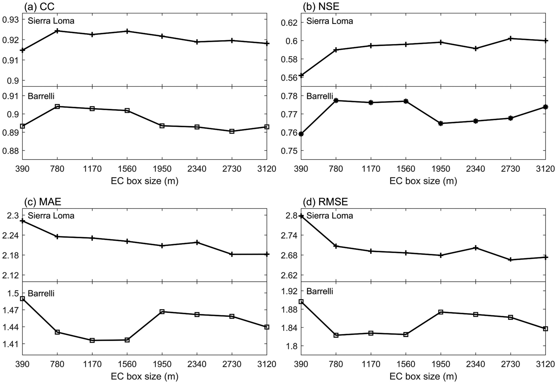
Fig. 9 illustrates sharpening performance in terms of four quantitative metrics: CC, NSE, MAE, and RMSE. We use varying ranges in the y-axes for the three sites to better highlight the variations of metrics. For the three study sites, the sharpening accuracy based on these metrics shows a relatively large increase as the EC box size increases from 90 m, indicating an enhanced performance of the modified DMS approach over the standard DMS in which the EC process was carried out at near native resolution scale (90 m). The overall behavior in performance metrics in Fig. 9 is similar to that of simulated experiments (Fig. 6) with shifts of 90 m, encompassing the maximum displacement identified in Section 4.1. This suggests that factors in addition to a linear shift are impacting the combined ECOSTRESS-Landsat sharpening in these cases, and the simulations in Fig. 6 represent a best-case misalignment scenario with same-platform datasets. Additional factors may include non-linear, spatially variable shifts (warping), differences in time-of-day and surface illumination, and differences in view angle. At large values of EC box size, the positive benefits of relaxing EC box size asymptote similar to the simulated experiment in Fig. 6 and the response of overlapped area to the EC box size in Fig. 3.

Fig. 9.

(a) CC, (b) NSE, (c) MAE and (d) RMSE between the sharpened 30-m Landsat 8 LST (reference) and 30-m ECOSTRESS LST with EC box size (m) over the Sierra Loma, Barrelli, and Ripperdan sites.

In comparison with the simulated experiment, the trends of sharpening accuracy with respect to EC box size in ECOSTRESS LST sharpening shows larger fluctuations, particularly at the Barrelli site which is characterized by significant topographic variability and attendant sensitivity to sun and view angle in both the thermal and reflectance bands. These fluctuations may also be linked to systematic LST differences between the ECOSTRESS and Landsat 8/UAV data due to overpass time difference and variable response among land covers with distinct thermal properties. CC shows lower fluctuations than other metrics because it is less sensitive to systematic LST differences resulting from diurnal changes and thus may be more reliable in evaluating the DMS algorithm.

In addition to the fluctuations, the magnitude of improvement of sharpening accuracy in terms of the four quantitative metrics for these real ECOSTRESS sharpening experiments (Fig. 9) is less significant than in the simulated experiment (Fig. 6), which represents a best-case scenario with scene-wide uniform shift and simultaneous TIR and VSWIR acquisition. Spatially varying shifts and differences in acquisition time in ECOSTRESS/Landsat imagery add noise that serves to reduce the realized improvement. Furthermore, it should be noted that the sub-scenes over which these statistics are computed, while heterogeneous and rich in structure, are dominated really by fields and natural vegetation patches that are internally homogeneous. The change of EC box size will have less impact on the sharpening results in these homogeneous patches compared to regions of discontinuity (e.g., field boundaries), which comprise a relatively small proportions of the statistical domains. The RMSE statistics average the results from all areas and understate the significance of the improvements of the modified DMS approach.

Still, the trends in the statistical metrics can be used in combination with visual evaluations to determine the optimal EC box size, as will be discussed in detail later. The following subsections show visual examples of sharpening results at the three test sites and discuss unique site-specific features of DMS performance.

4.3.1. Sierra Loma site

Fig. 10 shows a visual comparison of sharpened ECOSTRESS LST images over the Sierra Loma subset area using different EC box sizes with the reference sharpened Landsat LST image. While absolute temperature range differs between the Landsat and ECOSTRESS images due to different overpass times (accommodated by the greyscale stretch), the spatial patterns in the surface temperature fields are comparable between the two systems. The increasing clarity in sharpened ECOSTRESS LST images (Fig. 10c–i) demonstrates the effectiveness of the DMS technique for improving spatial detail and compatibility between sensors (Fig. 10b). Using the sharpened Landsat 8 LST (Fig. 10b) as reference, EC box sizes larger than 90 m result in much clearer field boundaries in the ECOSTRESS LST sharpening, as well as larger temperature contrast across the scene. Pixel-to-pixel scatterplots of sharpened ECOSTRESS LST vs. reference LST are shown in Fig. 11 for the subset area in Fig. 10. Scatter reduces around the best-fit regression line and correlation improves with EC box size up to about 450 m, as demonstrated in Fig. 9. The offset above the one-to-one line reflects systematic time-of-day-induced differences between the two LST fields and is expected.

Fig. 10.

(a) Landsat 30-m NIR-Red-Green composite for the 400 × 400 Sierra Loma study site subset on August 4, 2018; (b) sharpened 30-m Landsat 8 LST (reference; °C; left greyscale bar); (c) unsharpened ECOSTRESS LST resampled to 30-m resolution (°C; right greyscale bar); sharpened images of ECOSTRESS LST (°C; right greyscale bar) with (d) 90-m, (e) 180-m, (f) 270-m, (g) 360-m, (h) 450-m and (i) 540-m EC box size. Note that the colour bars are stretched to match LST contrast between sensors (Landsat: 25–55°C; ECOSTRESS: 30–55°C).

Fig. 11.

Scatter plots of the reference LST and sharpened ECOSTRESS LST over the Sierra Loma site with (a) 90-m, (b) 180-m, (c) 270-m, (d) 360-m, (e) 450-m and (f) 540-m EC box size.

Note, however, that by increasing the EC box size we are effectively forcing sharpened LST structure to resemble more and more the SR patterns, albeit using data-driven regressions developed near the native LST resolution. While the sharpened images may “look better” visually with large EC boxes, we may lose important LST signals in areas where the LST-SR relationship is atypical. The EC residuals in these discrepant areas can convey valuable information, for example recent irrigation or management activity (Anderson et al., 2004b). The goal is to select a nominal EC size that jointly minimizes impacts of registration errors while maximizing information content in the sharpened thermal image.

This choice is exemplified in the Sierra Loma subset region highlighted in Fig. 12, zooming in on a 6 × 6 km (200 × 200 30-m pixels) patch of irrigated agricultural land, specifically focusing on the fields indicated by a black box in the center of the scene. For the vegetated field (upper patch), a 90-m EC box allowed some bleeding of high LST from the adjacent bare field (lower patch) due to image misalignment. This bleeding is alleviated with larger boxes, with diminishing returns beyond 270 m. The correction afforded at that scale has important implications for the further use of sharpened LST for hydrological applications (e.g., evapotranspiration and crop water demand estimates) at sub-field to field scales.

Fig. 12.

(a) Landsat 30-m NIR-Red-Green composite for a 6 × 6 km subarea within the Sierra Loma domain (central point: 121°55′W, 39°42′N) on August 4, 2018; (b) sharpened 30-m Landsat 8 LST (reference; °C); sharpened images of ECOSTRESS LST (°C) with (c) 90-m, (d) 180-m, (e) 270-m, (f) 360-m, (g) 450-m and (h) 540-m EC box size.

4.3.2. Barrelli site

In comparison with Sierra Loma, the Barrelli site shows larger fluctuations in performance metrics in response to EC box size (Fig. 9). This is due in part to the smaller sample size used in sharpening resulting from the masking of ocean and smoke plume pixels. In addition, the large proportion of mountainous areas in the Barrelli scene will introduce variability due to the complex interactions between terrain shadowing and sensor overpass time differences.

Visual comparisons of reference and sharpened thermal images from Barrelli are illustrated in Fig. 13. Consistent with the Sierra Loma site, the original unsharpened LST (Fig. 13c) in Barrelli is much blurrier than the sharpened LST (Fig. 13d–i). Similar to the results based on quantitative metrics (Fig. 9), the visual comparison illustrates the benefits of relaxing EC box size beyond 90 m, in this case particularly in capturing the textures in the mountains. As with Sierra Loma (Figs. 10 and 12), EC box sizes above 180–270 m do not significantly improve visual clarity.

Fig. 13.

(a) Landsat 30-m NIR-Red-Green composite for the 400 × 400 Barrelli study site (central point: 122°59′W, 38°44′N) on August 11, 2018; (b) sharpened 30-m Landsat 8 LST (reference; °C; left greyscale bar); (c) unsharpened ECOSTRESS LST resampled to 30-m resolution (°C; right greyscale bar); sharpened images of ECOSTRESS LST (°C; right greyscale bar) with (d) 90-m, (e) 180-m, (f) 270-m, (g) 360-m, (h) 450-m and (i) 540-m EC box size.

4.3.3. Ripperdan site

Sharpening performance at Ripperdan was evaluated with respect to thermal imagery collected by the UAV over the GRAPEX vineyard sites (Fig. 14). While the UAV image extent is significantly smaller than the sharpened Landsat reference scenes used for evaluation at Sierra Loma and Barrelli, the 0.6 m native resolution of the thermal data affords direct assessment of thermal structures at 30 m. The lower correlations and higher RMSE and MAE at Ripperdan compared to the other sites, reported in Fig. 9, are partially due to the smaller sample size used to compute the statistics. In addition, differences in sensors and LST retrieval between the UAV and satellite datasets may contribute additional noise (Torres-Rua et al., 2019). For example, the lack of atmospheric correction to the UAV may account in part for the systematic underestimation of LST in comparison to ECOSTRESS data (Fig. 14b–c). RMSE is also inflated due to diurnal changes in surface temperature between the acquisition time of the UAV airborne data (12:34 PM, PST) and ECOSTRESS data (2:03 PM, PST). The unsystematic component of RMSE (RMSEu) is more comparable between sites (1.46–1.79 K; 1.24–1.32 K; 1.51–1.57 K over Ripperdan, Sierra Loma and Barrelli, respectively), suggesting a relatively large systematic RMSE that is very likely the primary reason for the negative NSE (not seen in the other two sites).

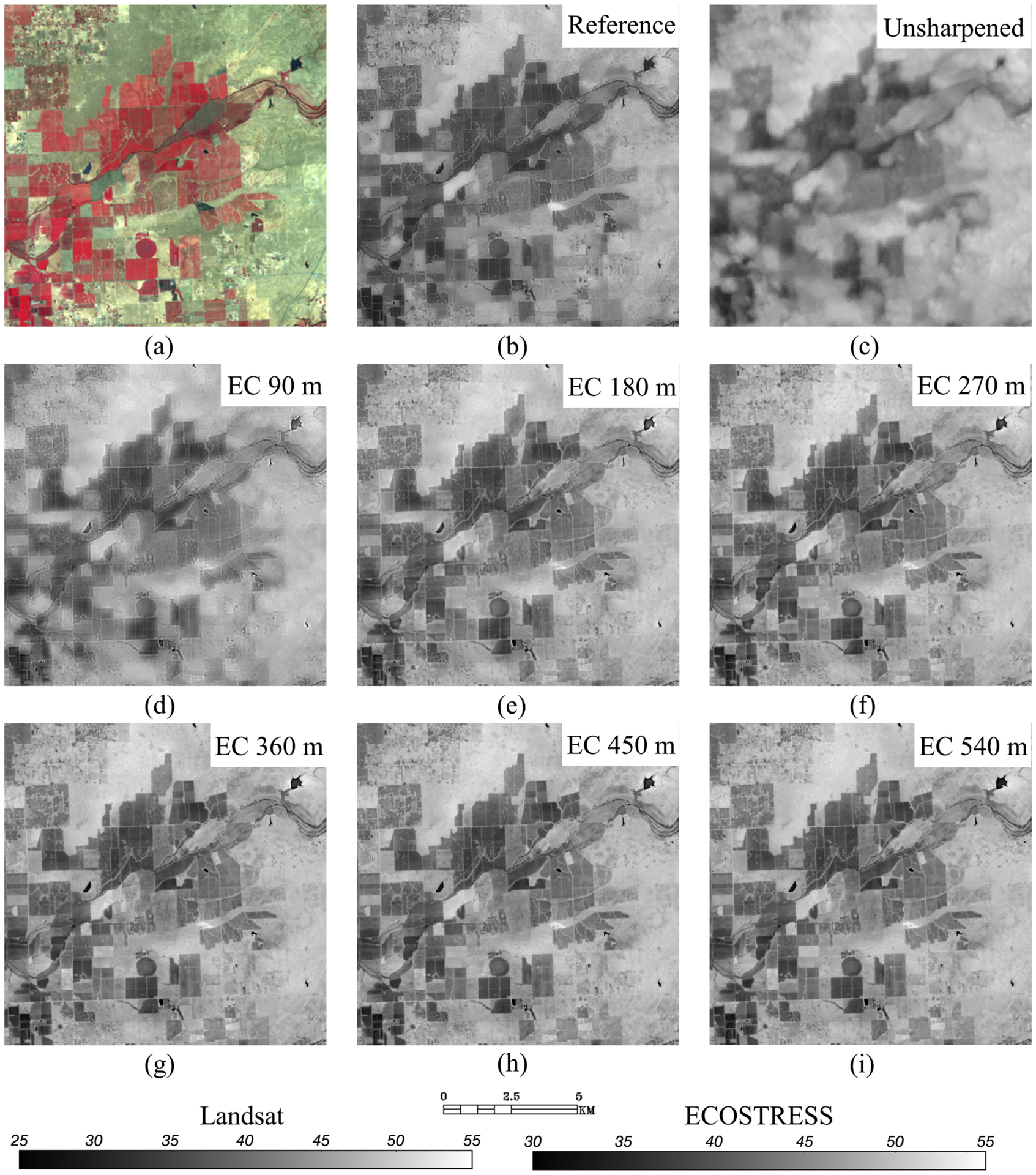
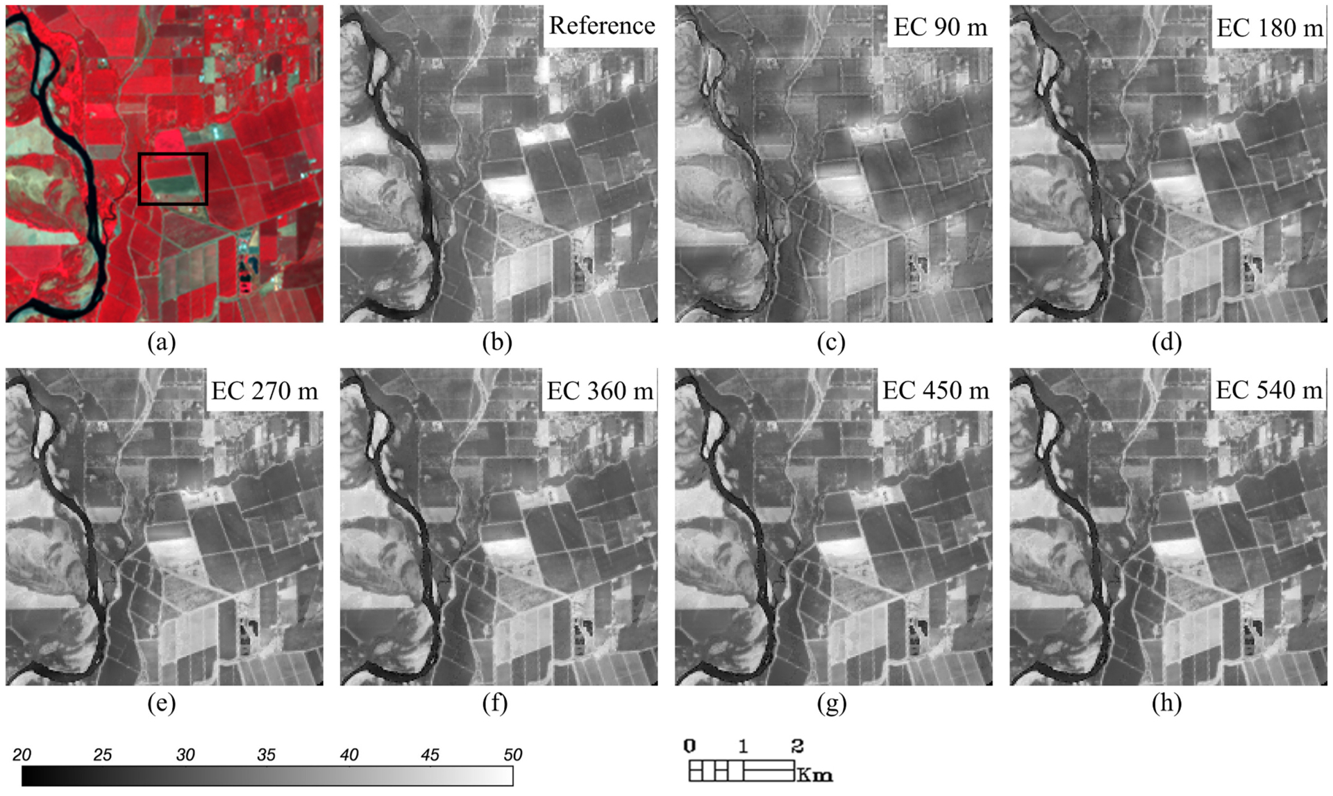
Fig. 14.

(a) HLS-S30 30-m NIR-Red-Green composite for the 146 × 85 Ripperdan study site (central point: 120°11′W, 36°50′N) on August 5, 2018; (b) resampled 30-m UAV LST (reference; °C; “UAV” greyscale bar); (c) unsharpened ECOSTRESS LST resampled to 30-m resolution (°C; “ECOSTRESS” greyscale bar); sharpened images of ECOSTRESS LST (°C; “ECOSTRESS” greyscale bar) with (d) 90-m, (e) 180-m, (f) 270-m, (g) 360-m, (h) 450-m and (i) 540-m EC box size; (j-o) residuals (°C; “Residual” greyscale bar) between (d-i) sharpened and (c) unsharpened images, respectively.

Fig. 14b–i provides a visual comparison of reference UAV LST imagery over Ripperdan and sharpened ECOSTRESS LST fields for EC box size ranging from 90 to 540 m with an interval of 90 m. For EC box sizes of 180 m and larger, temperature patterns more completely fill the field boundaries. For example, in the subset area indicated by the left-most black box (Fig. 14a), the LST image sharpened with a 90-m EC box (Fig. 14d) shows little temperature contrast between fields with denser (the left patch) and sparser vegetation (the right two patches). These contrasting thermal conditions seen in the UAV image are better defined at field scale with larger EC boxes (Fig. 14e–i).

As discussed in Section 4.3.1, excessively large EC box sizes may lead to loss of signal in features where the LST-SR relationship is atypical, and a reduced fidelity to the unsharpened LST. Residual maps, showing the differences between the sharpened and unsharpened ECOSTRESS LST at the 90-m pixel scale demonstrate the loss of fidelity with larger EC box size (Fig. 14j–o). In the subset area highlighted by the lower-right black box (Fig. 14a), the left-most field (vegetated) patch has a higher temperature in the unsharpened ECOSTRESS LST image than the two fields on the right (Fig. 14c). For EC boxes of 360 m and higher, this temperature contrast reverses in the sharpened images. This is highlighted by the increasing residuals in Fig. 14l–o. The constrast between unsharpened and sharpened image in these fields suggest that the impact of atypical LST-SR relationship may be amplified when the EC box size is large.

4.3.4. Site summary

Based on the collective sharpening results and analysis over the Sierra Loma, Barrelli, and Ripperdan sites, we recommend using an EC box size of 180–270 m for the ECOSTRESS LST sharpening. There are a few reasons for this choice. 1) The use of a relaxed EC box size of 180–270 m improves the sharpening accuracy over the use of 90 m (around the native resolution of ECOSTRESS). 2) The sharpening accuracy after 270 m gradually becomes insignificant with increased fluctuations and sometimes turns into a downward trend. 3) The relaxation of the EC box can lead to loss of spatial thermal detail, especially for large EC box sizes.

4.4. VIIRS LST sharpening

4.4.1. Selection of resampling strategy

Using the Sierra Loma site as a case study, we employed both NN and bilinear interpolation to resample the 375-m VIIRS swath LST data to the 30-m SR grid to study the impacts of gridding method on DMS sharpening. The relative performance of the two approaches was evaluated by comparing gridded unsharpened VIIRS LST against Landsat LST data in terms of CC and RMSEu. In addition, the gridded VIIRS LST data were also sharpened to 30-m resolution with both 390-m and 780-m EC box sizes and compared with sharpened Landsat LST. We selected two 400 × 400 subsets with different spatial patterns for the evaluation.

Fig. 15 indicates that the bilinear interpolation approach outperformed the NN approach for both the unsharpened and DMS sharpened cases, resulting in higher CC and lower RMSEu for both subsets. Relaxing the VIIRS EC box size from 390 to 780 m further improved statistical metrics. Based on these results, we adopted bilinear interpolation for LST swath resampling for use in the modified DMS approach. However, it should be noted that these experiments only represent a limited case, and more tests may be needed to identify which gridding/resampling approach is more generally suitable. In addition, it may be that these results are specific to the modified DMS approach, while other sharpening algorithms may benefit from a different gridding methodology.

Fig. 15.

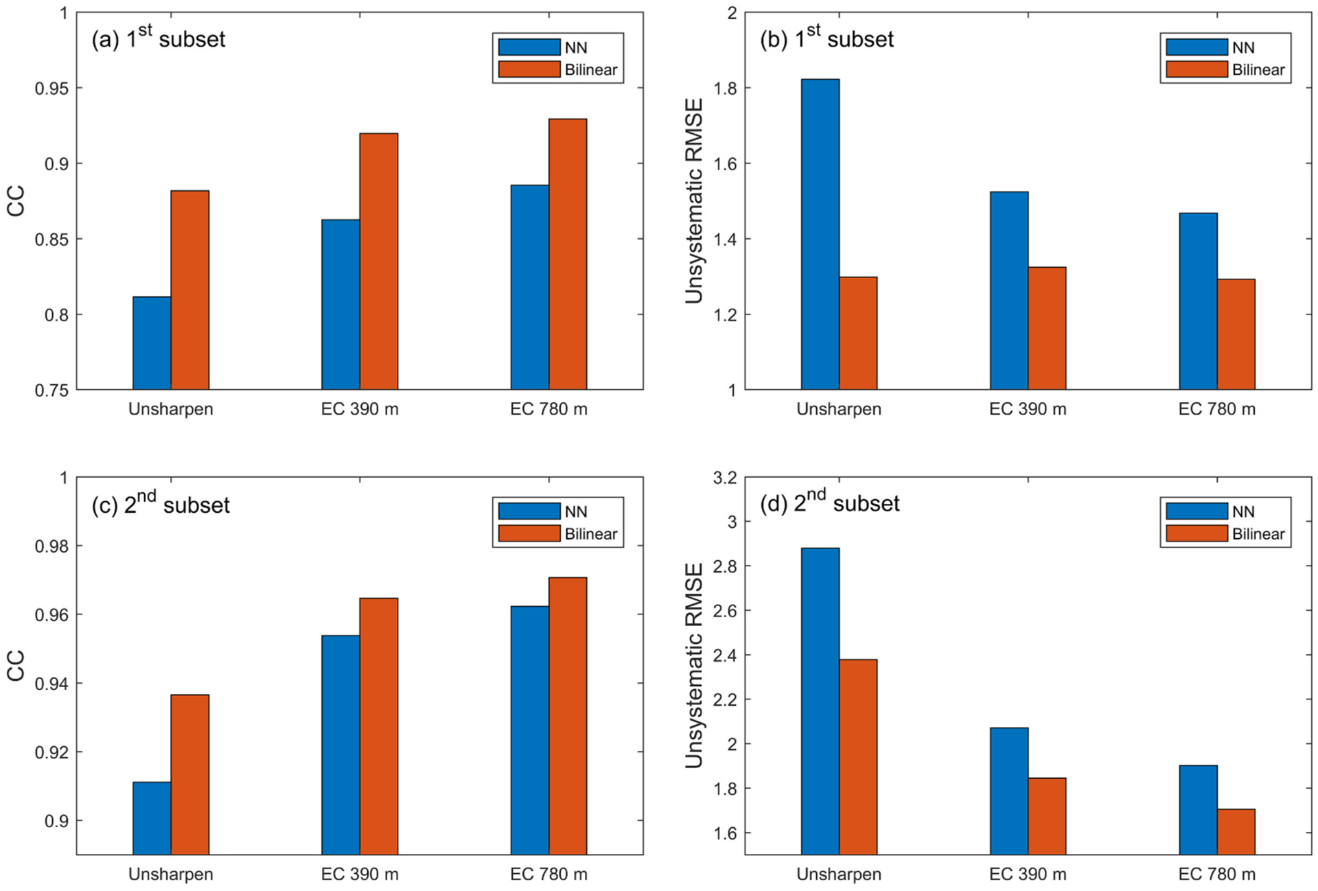
The evaluation of NN and bilinear resampling approaches in gridding LST data in terms of (a, c) CC and (b, d) RMSEu over two subsets in the Sierra Loma scene.

4.4.2. Sharpening evaluation

Evaluation of VIIRS LST sharpening using the modified DMS algorithm was conducted over the three study sites on the same dates as used in the ECOSTRESS analysis. The maximum image misalignment between VIIRS and Landsat 8/HLS (S30) data was found in Section 4.1 to be around 150 m, larger than that for ECOSTRESS (70 m). Therefore, based on the results from the simulated experiments, the optimal EC box size for VIIRS LST sharpening should be larger than that for ECOSTRESS. Considering the native resolution of VIIRS (375 m) and the larger registration errors, the range of EC box size used for testing VIIRS LST sharpening was set from 390 m to 3120 m with an interval of 390 m (integer multiples of the Landsat 30-m resolution).

The four quantitative measures of VIIRS sharpening accuracy for the prescribed set of EC box sizes are shown in Fig. 16. Over the Sierra Loma site, the experiment with a relaxed EC box size of 780 m produced an improved performance in comparison with a 390-m EC box based on the four metrics, consistent with sharpening via simulated-VIIRS LST (Fig. 8). As the EC box size continues to increase from 780 m, CC broadly indicates decreased sharpening accuracy. While the other three metrics point to increased accuracy, the change rate is relatively small. In general, 780 m appears to be a good candidate for the optimal EC box size. Another set of experiments with EC box size ranging from 450 to 720 m with a 90-m interval (figure not shown) did not identify a box size with CC or other performance metrics superior to the 780-m case, confirming to the selection of 780 m as the optimal EC size.

Fig. 16.

(a) CC, (b) NSE, (c) MAE and (d) RMSE between the sharpened 30-m Landsat 8 LST (reference) and the sharpened 30-m VIIRS LST with respect to a set of EC box sizes (m) over the Sierra Loma, Barrelli, and Ripperdan sites.

Assessment at the 30-m scale requires that both Landsat 8 and VIIRS LST are sharpened using the same 30 m Landsat 8 SR. To assess results independent of Landsat sharpening, another set of experiments was also conducted to sharpen the VIIRS LST to 90 m resolution over the Sierra Loma and Barrelli sites using Landsat 8 data at the native 100 m resolution as the reference. The results at 90 m (Fig. 17) are similar to those at 30 m (Fig. 16), and the same optimal EC box size (780 m) is identified.

Fig. 17.

(a) CC, (b) NSE, (c) MAE and (d) RMSE between the original 100-m Landsat 8 LST (reference) and sharpened VIIRS LST (90 m) with respect to a set of EC box sizes (m) over the Sierra Loma and Barrelli sites.

A visual comparison of the 30-m reference and sharpened VIIRS LST over a 12 × 12 km subarea in the Sierra Loma scene is provided in Fig. 18. The sharpening results using an EC box size near the native resolution of VIIRS (390 m) produced LST imagery with clear field boundaries in comparison, similar to the reference LST imagery (Fig. 18b). This is in contrast to ECOSTRESS LST sharpening in which the use of near-native resolution (90 m) for EC box size produced LST imagery with blurry field boundaries. This is because the scale gap between VIIRS LST and Landsat SR (375 m to 30 m) is much larger than that for the ECOSTRESS case (70 m to 30 m), whereas the maximum image misalignment is more comparable (150 m for VIIRS and 70 m for ECOSTRESS). For VIIRS LST sharpening, EC at the native spatial resolution is adequately large to produce imagery with clear field boundaries. The 780-m EC box case better reproduces some small-scale features in the Landsat LST map, such as the hot bare field just west of the center. Therefore, and considering the statistical metrics in Fig. 16, a good candidate for the optimal EC box size can be 780 m. Similar results were confirmed over the Barrelli and Ripperdan sites (not shown).

Fig. 18.

(a) Landsat 30-m NIR-Red-Green composite for the 400 × 400 Sierra Loma study site on August 4, 2018; (b) sharpened 30-m Landsat 8 LST (reference; °C; left greyscale bar); (c) unsharpened VIIRS LST resampled to 30-m resolution (°C; right greyscale bar); sharpened images of VIIRS LST (°C; right greyscale bar) with (d) 390-m, (e) 780-m, (f) 1170-m, (g) 1560-m, (h) 1950-m and (i) 2340-m EC box size.

4.5. Multi-source comparison of sharpening results

Integration of multi-source LST from ECOSTRESS, VIIRS, and Landsat provides an important path to improving the characterization of field-scale temporal variation in LST in comparison with using Landsat alone, facilitating frequent monitoring of land surface conditions for many applications. However, differences in spatial resolution between these satellite platforms do not allow easy stacking of multi-source LST data. The employment of the DMS algorithm in this study overcomes this difficulty by sharpening LST from different sources to a common spatial resolution. Based on the identified optimal EC box size for both ECOSTRESS (270 m) and VIIRS (780 m) in previous sections, we selected another subset area from the Sierra Loma and Barrelli domains (no Landsat for Ripperdan site) to visually demonstrate the ability of DMS to generate stackable LST fields from multiple thermal data sources. Fig. 19 shows comparisons between unsharpened and sharpened images for Landsat, ECOSTRESS and VIIRS over the two subset areas. The sharpening process brings the thermal images from all three sensors to a similar level of detail; however, we can see that the retrieval of detail is not perfect. In the Barrelli subset area, for example, there are some fields with higher temperatures in the northeast corner (highlighted in a black box) of Landsat and ECOSTRESS LST that are not apparent in VIIRS LST. These high-temperature features are at significantly subpixel scale within the unsharpened VIIRS image but are well captured by Landsat and ECOSTRESS at native resolution. It is very likely that these temperature anomalies are not well-related to SR and cannot be well reconstructed through the EC process in VIIRS LST sharpening. Still, the spatial textures in the three sharpened images are in general comparable and can be reasonably assembled into a stackable time series.

Fig. 19.

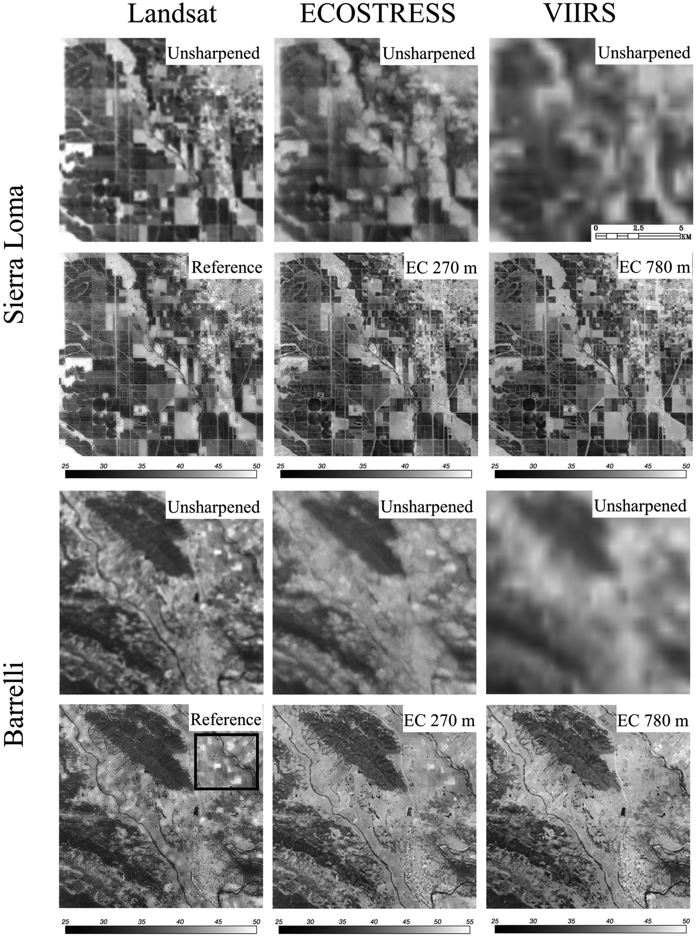
Visual comparisons between unsharpened (resampled to 30-m resolution) and sharpened images for Landsat (left column), ECOSTRESS (middle column) and VIIRS (right column) over a 400 × 400 subset of the Sierra Loma domain (top two rows; central point: 122°14′W, 39°42′N) on August 4, 2018, and the Barrelli domain (bottom two rows; central point: 122°53′W, 38°39′N) on August 11, 2018, respectively.

5. Discussion

In this study, we investigate the performance of multi-sensor data sharpening using TIR and SR data from the same date – a best-case scenario for sharpening, because the surface conditions have likely not changed significantly between band acquisition. For ECOSTRESS, there will be TIR acquisitions on dates when there is no commensurate VSWIR image acquisition (e.g., between Landsat and Sentinel-2 overpasses). While SR data from the closest overpass can be used, this can create challenges and add noise to the high-resolution LST reconstruction. Abrupt changes in surface conditions (e.g., irrigation, harvesting, deforestation, etc.) between sensor overpasses can corrupt the LST-SR relationship derived in DMS for LST sharpening. Even non-abrupt changes (e.g., rapid vegetation biomass accumulation during the growing season) can introduce errors in the sharpening process. The EC procedure adopted in the DMS approach can, to some extent, relieve the negative impact of these disturbances by adjusting the sharpened LST relative to the raw LST. Future work employing data from different dates is needed to further understand the algorithm performance.

The accuracy of LST sharpening ultimately depends on the underlying LST-SR model. Even if the SR and LST are acquired on the same day, the LST-SR relationship may not be able to capture all variabilities, particularly over areas with significant topography. The influence of topographic shadow changes induced by the interaction between complex terrains and sensor overpass time differences on LST-SR relationship can be spatially heterogeneous and thus contaminate the sharpening results at the scene scale. For example, the sharpening accuracy in the Barrelli site shows considerable fluctuations in response to EC size changes, which may be linked to the contaminating effect of the complex terrain and overpass time differences (10:51 am for Landsat, 12:04 pm for ECOSTRESS and 1:30 pm for VIIRS). To improve the sharpening, incorporation of more spectral band observations may be a useful path because it allows more information to characterize the LST-SR relationship. For instance, the three red-edge bands from the Sentinel-2 satellite that have not been used in this study are good candidates to be employed in future work and may have potential to improve sharpening results. In addition, a more advanced machine learning approach such as deep learning algorithms may improve the LST-SR model. This is important especially for a coarse resolution sensor such as VIIRS since LST spatial details mainly come from the LST-SR model. The threshold of c_v, an important parameter in building the LST-SR model, determines the relative homogeneity of an LST-SR sample at LST spatial resolution. In this study, we used c_v threshold of 0.1 for Landsat and ECOSTRESS and 0.2 for VIIRS. A different c_v threshold may be needed for other sensors for selecting sufficient and relatively homogeneous samples. Relaxing the EC size is a remedy for the misalignment between TIR and SWIR sensors from different satellite platforms. A better co-registration between sensors is needed for further improving LST sharpening.

6. Conclusion

In this study, the DMS approach, which has shown good performance for thermal sharpening based on data from a single platform, was employed to sharpen ECOSTRESS and VIIRS LST images using SR data from HLS products over three selected sites (Sierra Loma, Barrelli and Ripperdan site) in California. A modification to the standard DMS approach was investigated to address potential misregistration between SR and LST images collected on different platforms; namely, the relaxation of the spatial scale at which sharpened and unsharpened LST images are forced to match via the energy conservation step.

Based on shift experiments maximizing the correlation between NDVI and LST fields, typical subscene-scale misregistration between the ECOSTRESS and Landsat 8/HLS (S30) data used in this study was determined to be around 30–70 m and approximately 60–150 m for the VIIRS data. Results from the sharpening experiments demonstrate the superiority of modified DMS over standard DMS, suggesting the effectiveness of relaxing sampling window and EC box in reducing impacts due to the co-registration error among different satellites. Other factors (e.g., overpass time and data quality differences) that might impact the sharpening results were also discussed. The results from these experiments suggest five committees for cubist regression tree training, a 5 × 5/15 × 15 window for sampling process and an optimal EC box size of 180–270 m/780 m for ECOSTRESS/VIIRS LST sharpening are reasonably good candidates for future applications.

This study improves our understanding of the capability of the thermal sharpening approach in handling multi-source data and provides solutions to deal with the challenge facing such sharpening. The development of an operational DMS framework that can be applied routinely to HLS, ECOSTRESS and VIIRS data over a variety of landscapes is in progress. Future work will be aimed at using these multi-source LST images to generate evapotranspiration estimates with high temporal frequency and at sub-field spatial resolutions, for applications in monitoring of crop water use and stress.

References

- Agam N, Kustas WP, Anderson MC, Li F, Colaizzi PD, 2007a. Utility of thermal sharpening over Texas high plains irrigated agricultural fields. J. Geophys. Res. Atmos 112. [Google Scholar]
- Agam N, Kustas WP, Anderson MC, Li F, Neale CM, 2007b. A vegetation index based technique for spatial sharpening of thermal imagery. Remote Sens. Environ 107, 545–558. [Google Scholar]
- Agam N, Kustas WP, Anderson MC, Li F, Colaizzi PD, 2008. Utility of thermal image sharpening for monitoring field-scale evapotranspiration over rainfed and irrigated agricultural regions. Geophys. Res. Lett 35. [Google Scholar]
- Allen RG, Tasumi M, Trezza R, 2007. Satellite-based energy balance for mapping evapotranspiration with internalized calibration (METRIC)—model. J. Irrig. Drain. Eng 133, 380–394. [Google Scholar]
- Allen RG, Robison CW, Garcia M, Kjaersgaard J, Kramber W, 2008. Enhanced resolution of evapotranspiration by sharpening the Landsat thermal band. Proc. ASPRS Pecora 17. [Google Scholar]
- Allen R, Irmak A, Trezza R, Hendrickx JM, Bastiaanssen W, Kjaersgaard J, 2011. Satellite-based ET estimation in agriculture using SEBAL and METRIC. Hydrol. Process 25, 4011–4027. [Google Scholar]
- Anderson M, Neale C, Li F, Norman J, Kustas W, Jayanthi H, Chavez J, 2004a. Upscaling ground observations of vegetation water content, canopy height, and leaf area index during SMEX02 using aircraft and Landsat imagery. Remote Sens. Environ 92, 447–464. [Google Scholar]
- Anderson MC, Norman J, Mecikalski JR, Torn RD, Kustas WP, Basara JB, 2004b. A multiscale remote sensing model for disaggregating regional fluxes to micrometeorological scales. J. Hydrometeorol 5, 343–363. [Google Scholar]
- Anderson MC, Kustas WP, Norman JM, 2007. Upscaling flux observations from local to continental scales using thermal remote sensing. Agron. J 99, 240–254. [Google Scholar]
- Anderson M, Norman J, Kustas W, Houborg R, Starks P, Agam N, 2008. A thermal-based remote sensing technique for routine mapping of land-surface carbon, water and energy fluxes from field to regional scales. Remote Sens. Environ 112, 4227–4241. [Google Scholar]
- Anderson MC, Allen RG, Morse A, Kustas WP, 2012. Use of Landsat thermal imagery in monitoring evapotranspiration and managing water resources. Remote Sens. Environ 122, 50–65. [Google Scholar]
- Anderson M, Gao F, Knipper K, Hain C, Dulaney W, Baldocchi D, Eichelmann E, Hemes K, Yang Y, Medellin-Azuara J, 2018. Field-scale assessment of land and water use change over the California Delta using remote sensing. Remote Sens 10, 889. [Google Scholar]
- Anderson MC, Yang Y, Xue J, Knipper KR, Yang Y, Gao F, Hain C, Kustas WP, Cawse-Nicholson K, Hulley G, Fisher JB, Alfieri JG, Meyers T, Prueger J, Baldocchi D, Rey-Sanchez C, 2020. Interoperability of ECOSTRESS and Landsat for mapping evapotranspiration time series at sub-field scales. In: Remote Sensing of Environment, (in review). [Google Scholar]
- Berk A, Bernstein LS, Robertson DC, 1987. MODTRAN: A Moderate Resolution Model for LOWTRAN Spectral Sciences Inc, Burlington, MA. [Google Scholar]
- Bindhu V, Narasimhan B, Sudheer K, 2013. Development and verification of a non-linear disaggregation method (NL-DisTrad) to downscale MODIS land surface temperature to the spatial scale of Landsat thermal data to estimate evapotranspiration. Remote Sens. Environ 135, 118–129. [Google Scholar]
- Bisquert M, Sánchez JM, Caselles V, 2016. Evaluation of disaggregation methods for downscaling MODIS land surface temperature to Landsat spatial resolution in Barrax test site. IEEE J. Select. Topics Appl. Earth Observ. Remote Sens 9, 1430–1438. [Google Scholar]
- Bonafoni S, 2016. Downscaling of Landsat and MODIS land surface temperature over the heterogeneous urban area of Milan. IEEE J. Select. Topics Appl. Earth Observ. Remote Sens 9, 2019–2027. [Google Scholar]
- Bosilovich MG, Chen J, Robertson FR, Adler RF, 2008. Evaluation of global precipitation in reanalyses. J. Appl. Meteorol. Climatol 47, 2279–2299. [Google Scholar]
- Cammalleri C, Ciraolo G, Minacapilli M, 2008. Spatial sharpening of land surface temperature for daily energy balance applications. In: Remote Sensing for Agriculture, Ecosystems, and Hydrology X International Society for Optics and Photonics, pp. 71040J. [Google Scholar]
- Cao C, De Luccia FJ, Xiong X, Wolfe R, Weng F, 2013. Early on-orbit performance of the visible infrared imaging radiometer suite onboard the Suomi National Polar-Orbiting Partnership (S-NPP) satellite. IEEE Trans. Geosci. Remote Sens 52, 1142–1156. [Google Scholar]
- Chen X, Yamaguchi Y, Chen J, Shi Y, 2012. Scale effect of vegetation-index-based spatial sharpening for thermal imagery: a simulation study by ASTER data. IEEE Geosci. Remote Sens. Lett 9, 549–553. [Google Scholar]
- Chen X, Li W, Chen J, Rao Y, Yamaguchi Y, 2014. A combination of TsHARP and thin plate spline interpolation for spatial sharpening of thermal imagery. Remote Sens 6, 2845–2863. [Google Scholar]
- Claverie M, Ju J, Masek JG, Dungan JL, Vermote EF, Roger J-C, Skakun SV, Justice C, 2018. The Harmonized Landsat and Sentinel-2 surface reflectance data set. Remote Sens. Environ 219, 145–161. [Google Scholar]
- Cook M, Schott JR, Mandel J, Raqueno N, 2014. Development of an operational calibration methodology for the Landsat thermal data archive and initial testing of the atmospheric compensation component of a Land Surface Temperature (LST) product from the archive. Remote Sens 6, 11244–11266. [Google Scholar]
- Dominguez A, Kleissl J, Luvall JC, Rickman DL, 2011. High-resolution urban thermal sharpener (HUTS). Remote Sens. Environ 115, 1772–1780. [Google Scholar]
- Fisher J, Hook S, Allen R, Anderson M, French A, Hain C, Hulley G, Wood E, 2015. ECOSTRESS: NASA’s next-generation mission to measure evapotranspiration from the International Space Station. In: AGU Fall Meeting Abstracts [Google Scholar]
- Gao F, Kustas WP, Anderson MC, 2012. A data mining approach for sharpening thermal satellite imagery over land. Remote Sens 4, 3287–3319. [Google Scholar]
- Guzinski R, Nieto H, 2019. Evaluating the feasibility of using Sentinel-2 and Sentinel-3 satellites for high-resolution evapotranspiration estimations. Remote Sens. Environ 221, 157–172. [Google Scholar]
- Hulley G, Hook S, Fisher J, Lee C, 2017. Ecostress, a nasa earth-ventures instrument for studying links between the water cycle and plant health over the diurnal cycle. In: 2017 IEEE International Geoscience and Remote Sensing Symposium (IGARSS) IEEE, pp. 5494–5496. [Google Scholar]
- Hutengs C, Vohland M, 2016. Downscaling land surface temperatures at regional scales with random forest regression. Remote Sens. Environ 178, 127–141. [Google Scholar]
- Inamdar AK, French A, 2009. Disaggregation of GOES land surface temperatures using surface emissivity. Geophys. Res. Lett 36. [Google Scholar]
- Inamdar AK, French A, Hook S, Vaughan G, Luckett W, 2008. Land surface temperature retrieval at high spatial and temporal resolutions over the southwestern United States. J. Geophys. Res. Atmos 113. [Google Scholar]
- Jeganathan C, Hamm N, Mukherjee S, Atkinson PM, Raju P, Dadhwal V, 2011. Evaluating a thermal image sharpening model over a mixed agricultural landscape in India. Int. J. Appl. Earth Obs. Geoinf 13, 178–191. [Google Scholar]
- Kaheil YH, Rosero E, Gill MK, McKee M, Bastidas LA, 2008. Downscaling and forecasting of evapotranspiration using a synthetic model of wavelets and support vector machines. IEEE Trans. Geosci. Remote Sens 46, 2692–2707. [Google Scholar]
- Knipper KR, Kustas WP, Anderson MC, Alfieri JG, Prueger JH, Hain CR, Gao F, Yang Y, McKee LG, Nieto H, 2019. Evapotranspiration estimates derived using thermal-based satellite remote sensing and data fusion for irrigation management in California vineyards. Irrig. Sci 37, 431–449. [Google Scholar]
- Krause P, Boyle D, Bäse F, 2005. Comparison of different efficiency criteria for hydrological model assessment. Adv. Geosci 5, 89–97. [Google Scholar]
- Kustas W, Anderson M, 2009. Advances in thermal infrared remote sensing for land surface modeling. Agric. For. Meteorol 149, 2071–2081. [Google Scholar]
- Kustas WP, Norman JM, Anderson MC, French AN, 2003. Estimating subpixel surface temperatures and energy fluxes from the vegetation index–radiometric temperature relationship. Remote Sens. Environ 85, 429–440. [Google Scholar]
- Kustas W, Li F, Jackson T, Prueger J, MacPherson J, Wolde M, 2004. Effects of remote sensing pixel resolution on modeled energy flux variability of croplands in Iowa. Remote Sens. Environ 92, 535–547. [Google Scholar]
- Kustas WP, Anderson MC, Alfieri JG, Knipper K, Torres-Rua A, Parry CK, Nieto H, Agam N, White WA, Gao F, 2018. The grape remote sensing atmospheric profile and evapotranspiration experiment. Bull. Am. Meteorol. Soc 99, 1791–1812. [DOI] [PMC free article] [PubMed] [Google Scholar]
- Legates DR, McCabe GJ Jr., 1999. Evaluating the use of “goodness-of-fit” measures in hydrologic and hydroclimatic model validation. Water Resour. Res 35, 233–241. [Google Scholar]
- Lillo M, García-Pedrero A, Merino G, Gonzalo-Martin C, 2018. TS2uRF: A New Method for Sharpening Thermal Infrared Satellite Imagery
- Liu Y, Hiyama T, Yamaguchi Y, 2006. Scaling of land surface temperature using satellite data: a case examination on ASTER and MODIS products over a heterogeneous terrain area. Remote Sens. Environ 105, 115–128. [Google Scholar]
- Liu K, Su H, Li X, Chen S, Zhang R, Wang W, Yang L, Liang H, Yang Y, 2018. A thermal disaggregation model based on trapezoid interpolation. IEEE J. Select. Topics Appl. Earth Observ. Remote Sens 11, 808–820. [Google Scholar]
- Merlin O, Duchemin B, Hagolle O, Jacob F, Coudert B, Chehbouni G, Dedieu G, Garatuza J, Kerr Y, 2010. Disaggregation of MODIS surface temperature over an agricultural area using a time series of Formosat-2 images. Remote Sens. Environ 114, 2500–2512. [Google Scholar]
- Mukherjee S, Joshi PK, Garg RD, 2015. Regression-Kriging technique to downscale satellite-derived land surface temperature in heterogeneous agricultural landscape. IEEE J. Select. Topics Appl. Earth Observ. Remote Sens 8, 1245–1250. [Google Scholar]
- Nash JE, Sutcliffe JV, 1970. River flow forecasting through conceptual models part I—A discussion of principles. J. Hydrol 10, 282–290. [Google Scholar]
- Nichol J, 2009. An emissivity modulation method for spatial enhancement of thermal satellite images in urban heat island analysis. Photogramm. Eng. Remote. Sens 75, 547–556. [Google Scholar]
- Norman J, Anderson M, Kustas W, French A, Mecikalski J, Torn R, Diak G, Schmugge T, Tanner B, 2003. Remote sensing of surface energy fluxes at 101-m pixel resolutions. Water Resour. Res 39. [Google Scholar]
- Pereira OJR, Melfi AJ, Montes CR, Lucas Y, 2018. Downscaling of ASTER thermal images based on geographically weighted regression Kriging. Remote Sens 10, 633. [Google Scholar]
- Price JC, 1983. Estimating surface temperatures from satellite thermal infrared data—a simple formulation for the atmospheric effect. Remote Sens. Environ 13, 353–361. [Google Scholar]
- Rienecker MM, Suarez MJ, Gelaro R, Todling R, Bacmeister J, Liu E, Bosilovich MG, Schubert SD, Takacs L, Kim G-K, 2011. MERRA: NASA’s modern-era retrospective analysis for research and applications. J. Clim 24, 3624–3648. [DOI] [PMC free article] [PubMed] [Google Scholar]
- Roy DP, Wulder MA, Loveland TR, Woodcock C, Allen RG, Anderson MC, Helder D, Irons JR, Johnson DM, Kennedy R, 2014. Landsat-8: science and product vision for terrestrial global change research. Remote Sens. Environ 145, 154–172. [Google Scholar]
- Saha S, Moorthi S, Wu X, Wang J, Nadiga S, Tripp P, Behringer D, Hou Y-T, Chuang H. y., Iredell M, 2014. The NCEP climate forecast system version 2. J. Clim 27, 2185–2208. [Google Scholar]
- Saunders R, Hocking J, Turner E, Rayer P, Rundle D, Brunel P, Vidot J, Roquet P, Matricardi M, Geer A, Bormann N, Lupu C, 2018. An update on the RTTOV fast radiative transfer model (currently at version 12). Geosci. Model Dev 11, 2717–2737. [Google Scholar]
- Schueler CF, Lee TF, Miller SD, 2013. VIIRS constant spatial-resolution advantages. Int. J. Remote Sens 34, 5761–5777. [Google Scholar]
- Singh Rawat K, Sehgal V, Ray S, 2019. Downscaling of MODIS thermal imagery. Egypt. J. Remote Sens. Space Sci 22, 49–58. [Google Scholar]
- Sismanidis P, Keramitsoglou I, Bechtel B, Kiranoudis CT, 2017. Improving the downscaling of diurnal land surface temperatures using the annual cycle parameters as disaggregation kernels. Remote Sens 9, 23. [Google Scholar]
- Smyth M, Leprince S, 2018. ECOSTRESS level-1B resampling and geolocation algorithm theoretical basis document (ATBD). In: N.J.P.L.i.E.P. Document California Institute of Technology. [Google Scholar]
- Sun L, Anderson MC, Gao F, Hain C, Alfieri JG, Sharifi A, McCarty GW, Yang Y, Yang Y, Kustas WP, 2017. Investigating water use over the C hoptank R iver W atershed using a multisatellite data fusion approach. Water Resour. Res 53, 5298–5319. [Google Scholar]
- Torres-Rua AF, Ticlavilca AM, Bachour R, McKee M, 2016. Estimation of surface soil moisture in irrigated lands by assimilation of landsat vegetation indices, surface energy balance products, and relevance vector machines. Water 8, 167. [Google Scholar]
- Torres-Rua A, Nieto H, Parry C, Elarab M, Collatz W, Coopmans C, McKee L, McKee M, Kustas W, 2018. Inter-comparison of thermal measurements using ground-based sensors, UAV thermal cameras, and eddy covariance radiometers. In: Autonomous Air and Ground Sensing Systems for Agricultural Optimization and Phenotyping III International Society for Optics and Photonics, pp. 106640E. [DOI] [PMC free article] [PubMed] [Google Scholar]
- Torres-Rua A, Aboutalebi M, Wright T, Nassar A, Guillevic P, Hipps L, Gao F, Jim K, Alsina MM, Coopmans C, 2019. Estimation of surface thermal emissivity in a vineyard for UAV microbolometer thermal cameras using NASA HyTES hyperspectral thermal, and landsat and AggieAir optical data. In: Autonomous Air and Ground Sensing Systems for Agricultural Optimization and Phenotyping IV International Society for Optics and Photonics, pp. 1100802. [DOI] [PMC free article] [PubMed] [Google Scholar]
- Torres-Rua AF, Ticlavilca AM, Aboutalebi M, Nieto H, Alsina MM, White A, Prueger JH, Alfieri JG, Hipps LE, McKee LG, Kustas W, Coopmans C, Dokoozlian N, 2020. Estimation of evapotranspiration and energy fluxes using a deep learning-based high-resolution emissivity model and the two-source energy balance model with sUAS information. In: Autonomous Air and Ground Sensing Systems for Agricultural Optimization and Phenotyping V International Society for Optics and Photonics, pp. 114140B. [DOI] [PMC free article] [PubMed] [Google Scholar]
- Trezza R, Allen R, Robison C, Kramber W, Kjaersgaard J, Tasumi M, Garcia M, 2008. Enhanced resolution of evapotranspiration from riparian systems and field edges by sharpening the Landsat thermal band In: World Environmental and Water Resources Congress 2008: Ahupua’A, pp. 1–12. [Google Scholar]
- Wang W, Cao C, Bai Y, Blonski S, Schull M, 2017. Assessment of the NOAA S-NPP VIIRS geolocation reprocessing improvements. Remote Sens 9, 974. [Google Scholar]
- Willmott CJ, Ackleson SG, Davis RE, Feddema JJ, Klink KM, Legates DR, O’donnell J, Rowe CM, 1985. Statistics for the evaluation and comparison of models. J. Geophys. Res. Oceans 90, 8995–9005. [Google Scholar]
- Wolfe RE, Lin G, Nishihama M, Tewari KP, Montano E, 2012. NPP VIIRS early on-orbit geometric performance. In: Earth Observing Systems XVII International Society for Optics and Photonics, pp. 851013. [Google Scholar]
- Wolfe RE, Lin G, Nishihama M, Tewari KP, Tilton JC, Isaacman AR, 2013. Suomi NPP VIIRS prelaunch and on-orbit geometric calibration and characterization. J. Geophys. Res. Atmos 118, 11,508–511,521. [Google Scholar]
- Yang Y, Anderson M, Gao F, Hain C, Kustas W, Meyers T, Crow W, Finocchiaro R, Otkin J, Sun L, 2017a. Impact of tile drainage on evapotranspiration in South Dakota, USA, based on high spatiotemporal resolution evapotranspiration time series from a multisatellite data fusion system. IEEE J. Select. Topics Appl. Earth Observ. Remote Sens 10, 2550–2564. [Google Scholar]
- Yang Y, Anderson MC, Gao F, Hain CR, Semmens KA, Kustas WP, Noormets A, Wynne RH, Thomas VA, Sun G, 2017b. Daily Landsat-scale evapotranspiration estimation over a forested landscape in North Carolina, USA, using multi-satellite data fusion. Hydrol. Earth Syst. Sci 21, 1017–1037. [Google Scholar]
- Yang Y, Cao C, Pan X, Li X, Zhu X, 2017c. Downscaling Land Surface Temperature in an Arid Area by Using Multiple Remote Sensing Indices with Random Forest Regression
- Yang Y, Anderson MC, Gao F, Wardlow B, Hain CR, Otkin JA, Alfieri J, Yang Y, Sun L, Dulaney W, 2018. Field-scale mapping of evaporative stress indicators of crop yield: an application over Mead, NE, USA. Remote Sens. Environ 210, 387–402. [Google Scholar]
- Zakšek K, Oštir K, 2012. Downscaling land surface temperature for urban heat island diurnal cycle analysis. Remote Sens. Environ 117, 114–124. [Google Scholar]
- Zhu Z, Woodcock CE, 2012. Object-based cloud and cloud shadow detection in Landsat imagery. Remote Sens. Environ 118, 83–94. [Google Scholar]