

Abstract
In recent years there has been much progress on the investigation of the QCD phase diagram with lattice QCD simulations. In this review we focus on the developments in the last two years. Especially the addition of external influences or new parameter ranges yields an increasing number of interesting results. We discuss the progress for small, finite densities from both extrapolation-based methods (Taylor expansion and analytic continuation for imaginary chemical potential) and complex Langevin simulations, for heavy quark bound states (quarkonium), the dependence on the quark masses (Columbia plot) and the influence of a magnetic field. Many of these conditions are relevant for the understanding of both the QCD transition in the early universe and heavy ion collision experiments, which are conducted for example at the LHC and RHIC.
Introduction
The strong interaction between quarks and gluons in the standard model is described by Quantum Chromo Dynamics (QCD). The investigation of the phase diagram of QCD has been an active subject for many years. A special focus of this research is on the transition between hadrons at low temperature and the quark–gluon plasma at high temperature. The nature of the transition as an analytic crossover (Refs. [1–6]) has been known since 2006 (Refs. [1, 2]). However, different external influences may change the nature of this transition. One famous example is the addition of a chemical potential. The crossover has been established for vanishing baryon chemical potential only, which means: for a setting with the same number of quarks and anti-quarks. This setting is a good approximation for the QCD transition in the early universe. However, the experimental investigations of the QCD transition rely on heavy ion collision experiments which produce the quark–gluon plasma with a finite density. In addition, the collided matter goes through several stages and is not permanently in an equilibrium. Since, at the moment, full QCD cannot be solved under such conditions one has to take other paths. Certain parameter ranges can be described efficiently by effective theories. For other situations we depend on phenomenological models, which in turn require input information that can be gained from lattice simulations.
The progress on the phase diagram from lattice QCD corresponds well with, and is in part triggered by, an increasing number of available experimental results. At the moment most experimental results for heavy ion collision experiments are generated either by the Large Hadron Collider (LHC) at CERN in Geneva, Switzerland, or the Relativistic Heavy Ion Collider (RHIC) at the Brookhaven national laboratory in New York, USA. While the results form the LHC are at low densities, RHIC accesses information for a larger chemical potential. However, there are several upcoming facilities that will allow one to reach even higher densities. Some of them are for example the Nuclotron-based Ion Collider fAcility (NICA) at the Joint Institute for Nuclear Research (JINR) in Dubna, Russia, the Compressed Baryonic Matter Experiment (CBM) at the Facility for Antiproton and Ion Research in Europe (FAIR) at Darmstadt, Germany, and the J-PARC heavy ion project (J-PARC-HI) at the Japan Proton Accelerator Research Complex (J-PARC) in Tokai, Japan.
After this introduction, we will briefly describe the stages of a heavy ion collision experiment in Sect. 2. Linking lattice QCD to heavy ion collision experiments requires results at low finite density which we discuss in Sect. 3. The main challenge in this parameter range is the infamous sign problem which is discussed in Sect. 3.1. For continuum extrapolated, physical results, one therefore has to rely on extrapolations (Sect. 3.2) from vanishing (Taylor method) or imaginary chemical potential. One method that is getting relatively close to direct lattice simulations at finite density is complex Langevin simulations, which are therefore reviewed in Sect. 3.3. Other methods that are not discussed in this review are for example reweighting techniques [7–10], density of state methods [11, 12], using the canonical ensemble [13–15], formulations with dual variables [16] or Lefschetz thimbles [17, 18].
Another way to gain information on finite density QCD is discussed in Sect. 4, on lattice simulations of effective field theories. Here, we focus, with Sect. 4.1, on the results for heavy quark bound states, the so-called heavy quarkonium.
Despite the importance at finite density, also for zero density there are interesting influences to consider. One of them is the dependence of the transition type on the quark masses. It is often summarized in the Columbia plot, which is discussed in Sect. 5. The most interesting areas of the Columbia plot are the upper right (Sect. 5.5) and lower left corner (Sect. 5.1). Due to the low quark masses, and the resulting expensive computations, different tactics are employed in the study of the lower left corner of the Columbia plot. In this review we discuss the use of an imaginary chemical potential in Sect. 5.2 and the variation of the number of quark flavors in Sect. 5.3. Due to the lack of continuum extrapolated results in this parameter range, we provide an overview over the numbers obtained from different lattice actions and lattice spacings in Sect. 5.4.
There have been found many results for yet another region. The addition of a magnetic field to finite temperature QCD does not suffer from the sign problem and is also relevant for the understanding of heavy ion collision experiments. The progress recently made on our understanding of the phenomena triggered by a magnetic field is discussed in Sect. 6.
Finally, this review closes with a conclusion. Here we hope to convince the reader that finite temperature lattice QCD and especially the investigation of the QCD phase diagram is a fascinating, thriving topic, of which we can only cover parts in this review.
Heavy ion collisions
As the experimental realization of QCD thermodynamics is strongly linked with heavy ion collision experiments, we will take a small detour to explain the different stages occurring during such a collision, which are depicted in Fig. 1. In a heavy ion collision various nuclei can be used. Prominent examples are gold and lead, which have been used at RHIC and LHC. Two beams of nuclei are accelerated to relativistic velocities.
Fig. 1.
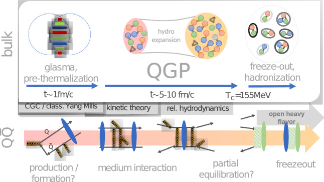
(Ref. [19]) Overview of the different stages of a heavy ion collision. In gray the different effective theories are shown which are used to describe the different stages (see Sect. 4.1)
When the two beams collide, they form a non-thermalized state with strongly interacting fields, which is called a glasma and commonly treated in the color glass condensate framework (for details on this framework see Refs. [20, 21]). Here the glasma is seen in the infinite momentum framework where there are partons of the nuclei, valence quarks and pairs of sea quarks. A main challenge is the description of different momentum scales. Due to the un-thermalized nature of this state, it is not accessible for lattice QCD simulations.
In the next stage, the further fragmentation of the partons into quarks and gluons leads to the quark–gluon plasma. This is a strongly interacting state of deconfined quarks and gluons. While first it was expected to be similar to an electromagnetic plasma, by now it is well established that it is more similar to a strongly interacting fluid. Therefore, it is often described by relativistic hydrodynamics.
The quark–gluon plasma expands and cools down at the same time. When it reaches temperatures close to the QCD transition temperature, the deconfined quarks and gluons have to recombine to color-neutral hadrons. At this time, the chemical abundance of the hadrons is determined. The corresponding temperature is called the chemical freeze-out temperature. However, the hadrons can still exchange energy and momentum until the point where the kinetic freeze-out takes place.
An important question is whether, at the stage of the quark–gluon plasma and the following transition to hadrons, the states thermalize. Only if this is the case, results from lattice QCD, which simulates thermal equilibrium, are directly applicable.
Low Finite density
One representation of the QCD phase diagram is in the T–-plane (Fig. 2). The axis is well investigated by lattice QCD. For low chemical potential and temperature, there is a hadronic phase of color-neutral bound states. At high temperatures the effective degrees of freedom are the quarks and gluons. This phase is called the quark–gluon plasma. These two phases are separated by a crossover at low and zero chemical potential. The transition is expected to change into a first order transition for higher with a critical second order point in between. The position of the critical point is under active investigation both by heavy ion collision experiments and by theoretic calculations. For very large chemical potentials, further fascinating phenomena, like a color superconducting phase [22], are expected.
Fig. 2.

A schematic view on the T–-plane of the QCD phase diagram
To analyze the quark–gluon plasma that is created in heavy ion collision experiments at the LHC or RHIC, a theoretical understanding of the quark–gluon plasma in QCD is needed. In the region of the deconfinement transition, QCD cannot be studied with perturbative methods. To get non-perturbative results with a controlled error, one has to turn to lattice QCD. At the moment, direct simulations that are continuum extrapolated and at physical quark masses are restricted to vanishing or imaginary chemical potential due to the infamous sign problem. On the other hand, the collisions especially at RHIC and upcoming heavy ion collision facilities like Fair and NICA take place away from the axis of zero . Therefore, information in that region is needed.
The sign problem
For simulation without chemical potential there are on average the same number of particles and antiparticles. Therefore, the expectation value of the overall baryon number density is zero. To describe a system with finite baryon density, we need to introduce a finite quark chemical potential into the Lagrangian. In the continuum this is relatively simple to achieve: by adding a term of the form . However, on the lattice, it is not that simple. Adding a similar term to the Dirac operator leads to a divergent energy density in the continuum limit, which is clearly unphysical. Instead one follows the idea of Hasenfratz and Karsch in [23] where the chemical potential is understood as the temporal component of a vector field. The temporal hopping term has then the form
| 1 |
It recovers the original action for and with it reproduces the correct density term at linear order in . However, this term breaks the -hermiticity of the Dirac operator,
| 2 |
and leads to a complex fermion determinant for real . The fermion determinant enters in the Boltzmann weight factor which has to be positive to allow for a Monte Carlo simulation. There have been several ideas on how to obtain results at real finite chemical potential, like reweighting techniques [7–10], Taylor expansion [24–28], density of state methods [11, 12], using the canonical ensemble [13–15], formulations with dual variables [16], Lefschetz thimbles [17, 18] or using a complex Langevin simulation [29, 30].
Extrapolation to finite
Instead of conducting direct simulations, for small densities it is possible to obtain results with physical quark masses by extrapolation. Since at the transition is a crossover (Refs. [1–6]), certain observables can be parameterized by an analytic function in the vicinity of zero as well. This fact can be exploited, by using results at zero (Refs. [24–28, 31–39]) or imaginary chemical potential (Refs. [38, 40–53]), to find a function that can be extrapolated to real, positive chemical potential. If one aims at gaining information from zero chemical potential, one uses the higher order derivatives of the partition function to calculate the Taylor coefficients of an expansion that can be continued to finite . This method is therefore often called the Taylor method.
The other possibility to determine a function that can be continued to finite chemical potential is the use of simulations at purely imaginary chemical potential, where there is no sign problem. As illustrated in Fig. 3, the data points can be described by a function of . For imaginary chemical potential this is the area where simulation results are available. The resulting data points can then be fitted with a function which can be extrapolated to and therefore to real, positive chemical potential. Since not much knowledge of the concrete shape of the describing function is available, the choice of the fit function influences the result at real chemical potential. Figure 3 shows three different fit functions, namely
| 3 |
| 4 |
| 5 |
each having three fit parameters, a, b, c. All three functions describe the available data well. However, their continuation to varies, especially for a temperature of MeV. This variation has, therefore, to be taken into account as a systematic error.
Fig. 3.

(Ref. [54]) Illustration of the analytic continuation from imaginary chemical potential. Data points generated with purely imaginary can be fitted as a function in and then extrapolated from to
When utilizing simulations at imaginary chemical potential, one exploits the fact that the -hermicity of the Dirac operator with a chemical potential reads
| 6 |
This means that in the action, the term adding the chemical potential is replaced by when switching to purely imaginary . For the determinant this yields
| 7 |
meaning that the determinant is only real if
| 8 |
For real f this is only fulfilled if , and, therefore, . However, if is chosen to be purely imaginary, this yields
| 9 |
Thus the determinant is real for a purely imaginary chemical potential. When using simulations at imaginary chemical potential, fewer derivatives are needed than for the Taylor method. Instead, one uses different fit functions to describe a data set for several imaginary chemical potentials. This method is sometimes called analytical continuation, but, since also the Taylor method relies on an analytical continuation, we will refer to it as the imaginary chemical potential method. The different fit functions can lead to different results which leads to the requirement of a careful systematic analysis. The behavior of one type of fit functions, the Padé approximation, is discussed in Ref. [55].
The transition temperature:
A common observable to extrapolate is the transition temperature. Because of the crossover nature of the transition, its definition is ambiguous. Typical definitions are, for example, the peak of the chiral susceptibility as a function of the temperature or the inflection point of the chiral condensate. Often different definitions yield consistent results within the available precision. However, for an analytic transition this is not guaranteed, in contrast to the situation for a phase transition.
A high precision determination of the transition temperature at from five different observables was done in Ref. [56]. As can be seen in Fig. 4, the five definitions have the same continuum limit within the available precision. This yields a combined value of MeV.
Fig. 4.
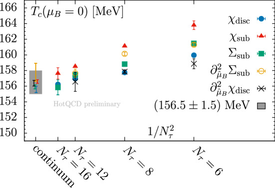
(Ref. [56]) The continuum extrapolation of five different definitions of the transition temperature. Towards the continuum limit the different definitions converge, yielding a combined result of MeV
A new definition as the peak of the chiral susceptibility as a function of the chiral condensate (instead of the more common definition as a function of the temperature) was introduced this year in Ref. [53]. It allows for a precise extraction of the transition temperature and, therefore, also for an improvement in the extrapolation. The results obtained from simulations at imaginary chemical potential are shown in Fig. 5. They are continuum extrapolated from the three lattices with sizes , and . The extrapolation was done with two different functions,
| 10 |
and
| 11 |
The transition temperature from imaginary chemical potential (Analytical continuation in the top of Fig. 5) is compared to the Taylor expansion at leading and next to leading order, and to results from truncated Dyson–Schwinger equations (Ref. [57]) and various determination of the chemical freeze-out temperature in heavy ion collision experiments (Refs. [58–62]).
Fig. 5.

(Ref. [53]) Top: A comparison between the extrapolated transition temperature obtained from analytical continuation from imaginary chemical potential with different functions, compared to the result from extrapolating with the leading order (LO) order next to leading order (NLO) Taylor coefficients. Bottom: A comparison of the extrapolated transition temperature to recent results from calculations with Dyson–Schwinger equations [57] and the freeze-out temperature from heavy ion collision experiments [58–62]
The transition temperature at finite chemical potential normalized by the transition temperature at zero chemical potential is often parameterized by
| 12 |
While there is a long history of the determination of [28, 38–40, 46, 47], results for [36, 53] only recently became available, from both the Taylor and the imaginary potential methods. It emerges that is significantly smaller than . Within its error it is still compatible with zero. A comparison of the recent determinations of both and is shown in Fig. 6.
Fig. 6.
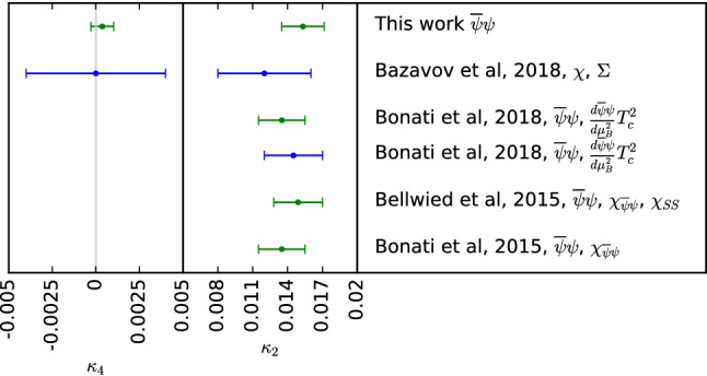
(Ref. [53]) A comparison of recent results for and as defined in equation (12). Reference [36] and the lower point of Ref. [38] use the Taylor method and are depicted in blue. The green points, which are the result from Ref. [53], the upper point of Refs. [38, 46, 47] used lattice data at imaginary chemical potential
Instead of an expansion in the baryon chemical potential, expansions in isospin, strangeness or charge chemical potential are also an option. They were studied in detail in Ref. [36]. There are two very similar possibilities to choose and for the expansion in that are commonly used. The first is the choice of a purely baryon chemical potential (). These conditions have been used in Ref. [46]. The second possible choice is the set up at the strangeness neutral point. In this case and are chosen in such a way that and to match the conditions in heavy ion collision experiments. This was done in Refs. [38, 47]. In all cases the two values agree within the error.
Fluctuations: Higher order fluctuations of conserved charges are calculated as the partial derivatives of the pressure (or the QCD partition function) with respect to the chemical potentials. Here,
| 13 |
with . These fluctuations are of great interest in the search for the critical endpoint, both for heavy ion experiments and theoretical calculations (Refs. [63–65]). They are proportional to powers of the correlation length and, therefore, they are expected to diverge in the vicinity of a critical end point (Resf. [26, 66–68]). Up to the eighth order fluctuations have been calculated on finite lattices in Refs. [31, 48, 52, 69]. The baryon fluctuations up to eighth order from Ref. [52] are shown in Fig. 7.
Fig. 7.
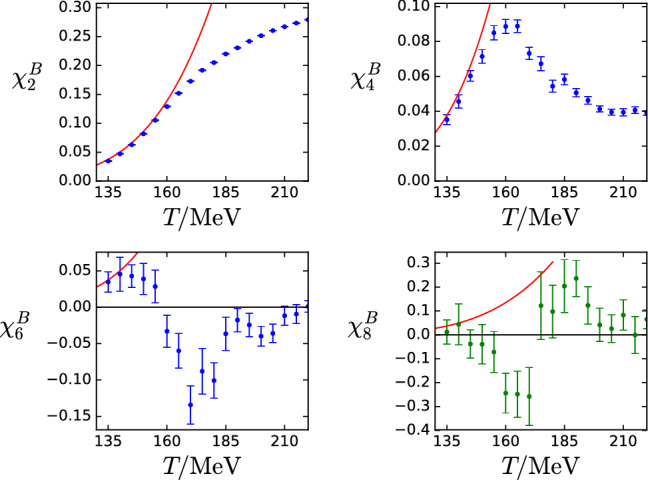
(Ref. [52]) Results for , , and an estimate for on a lattice as functions of the temperature, obtained from the single-temperature analysis (see text). We plot in green to point out that its determination is guided by a prior, which is linked to . The red curve in each panel corresponds to the results from the Hadron Resonance Gas model
In principle, fluctuations can also be measured both on the lattice and experiments. A comparison between theoretical and experimental results can be used to extract the chemical freeze-out temperature and the corresponding chemical potential as functions of the collision energy (Refs. [70–74]). To compare to experiments, one uses ratios of fluctuations to cancel out the explicit volume dependence. These can be matched to the ratios of cumulants of particle number distributions in experiments. However, not all baryons can be measured in experiments. Therefore, the cumulants of the proton number distribution are considered a useful proxy to compare to the baryon number cumulants calculated on the lattice. Some combinations are
| 14 |
| 15 |
| 16 |
| 17 |
| 18 |
where the mean , the variance , the skewness , the kurtosis , the hyper-skewness and the hyper-kurtosis are the first to sixth order moments of the baryon number distribution.
New results on continuum estimates for , and from lattice sizes and have been recently presented in Ref. [37]. For the comparison with experimental data along the transition line, and are shown (see top of Fig. 8) as a function of . Therefore, it is not necessary to determine the temperature and chemical potential in a heavy ion collision separately. This allows for a comparison with data from the STAR collaboration (Refs. [75, 76]). The experimental datapoints fit the lattice results well.
Fig. 8.

(Ref. [37]) Top: The ratios and as a function of evaluated along the transition line in comparison to the data from the STAR collaboration (Refs. [75, 76]). The lattice calculation is a continuum estimate from and lattices. Bottom: The ratios and as a function of evaluated along the pseudo-critical line in comparison to the data from the STAR collaboration (Ref. [76]). The lattice determination was done on an lattice
First calculations of the fifth and sixth order cumulants from a lattice are presented in the same way at the bottom of Fig. 8. Here only preliminary experimental data (Ref. [76]) is available for a comparison with . While errors are still large, both on the lattice and the experimental side, there seems to be a tension between both data sets. Changing the lattice results such that they can describe the two available experimental points would require unexpectedly large higher order corrections.
In general, a detailed comparison between lattice data and experiment requires the incorporation of many different aspects (Refs. [60, 78–80]). While on the lattice site, clearly, a continuum extrapolation is still needed, on the experimental side it is not always clear which particle species allow for good comparisons to the conserved charges measured in lattice QCD. While for the cumulants for the baryon number distribution the proton number distribution has been established as a reasonable proxy, for the strangeness number distribution the situation is less clear. A recent study in the hadron resonance gas (Ref. [77]) investigated different possibilities to find comparable observables. The comparison for different experimental proxies to the total, which would be the lattice result for , is shown in Fig. 9. The lattice prediction for is calculated on an lattice with two different methods. We have one that is based on the Taylor expansion and one that is based on the sector expansion (see Ref. [50]), where the pressure is parameterized as
| 19 |
As can be seen in Fig. 10, both expansions agree well for small chemical potentials and temperatures around 140 MeV. For higher temperatures, a deviation between the two methods becomes visible before the errorbar grows due to the increased chemical potential. Also the influence of different experimental cuts has been investigated.
Fig. 9.
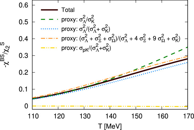
(Ref. [77]) Comparison between different possible combinations of particle number cumulants that could be measured experimentally (proxies) and the total of that could be determined in lattice QCD calculations. Both calculated in the Hadron Rasonance Gas model
Fig. 10.

(Ref. [77]) Comparison between the Taylor and the sector method for on an lattice, as well as results from the hadron resonance gas model (HRG)
The critical endpoint: To look for a bound on the critical endpoint in the QCD phase diagram, one can try to calculate the radius of convergence of an expansion in around . When one wants to estimate the radius of convergence naively from the fluctuations, one defines
| 20 |
If converges, in the limit of , it is guaranteed that there is no criticality within this radius. This has been done in Ref. [35] for the fluctuations up to sixth order.
However, it has been shown in Ref. [81] that the ratio estimator as given in Eq. (20) is never convergent in a finite volume. This is consistent with the fact that there is never a true phase transition in a finite volume. However, the convergence of the ratio estimator is problematic even when using the is extrapolated to infinite volume. It will work if one uses infinite-volume Taylor coefficients and the singularity determining the radius of convergence corresponds to a real phase transition in the infinite-volume limit. In the same work, alternative estimators have been discussed. Figure 11 shows results on an lattice for the standard estimator defined in Eq. (20), the modified Mercer–Roberts estimator
| 21 |
and the doubled index estimator
| 22 |
for a Taylor series with coefficients .
Fig. 11.

(Ref. [81]) The radius of convergence from three different estimators determined on an lattice. The green arrow indicates the result from reweighting
Another way to look for a critical endpoint and find the radius of convergence is the investigation of the Lee–Yang zeros (Ref. [82]). These are the zeros of the partition function in the plane of complex chemical potential. The radius of convergence is the distance to the closest (leading) Lee–Yang zero in the infinite Volume limit. If this happens to be on the real axis, it is a signal for the critical endpoint. While the higher order fluctuations needed for a reliable radius of convergence estimate suffer from increasingly larger errors and are difficult to determine, Ref. [81] discusses a cancelation that allows for a calculation of the leading Lee–Yang zero. However, this benefit holds only if it is possible to reweight by using a reduced matrix formulation (Refs. [9, 83–86]). This is not possible for the case of rooted staggered fermions. For this case, Ref. [87] introduces a new definition of the rooted staggered determinant, which allows for a numerical study of the Lee–Yang zeros. It is then tested on an lattice with stout smeared staggered fermions and a Symanzik improved gauge action. Spatial lattice extents of and 12 are used to estimate the infinite-volume limit. However, this approach might still suffer from the overlap problem related with reweighting.
In Ref. [88], an algorithm called sign-reweighting is proposed, aiming to avoid uncontrolled systematics like the overlap problem. This approach separates the sign of the Dirac determinant from the configuration generation which is done with a weight of . The sign is handled separately by a discrete reweighting.
Complex Langevin
One way to conduct lattice simulations, despite the sign problem that made significant progress, is by complex Langevin simulations. I will only give a very brief overview over the new developments. A more comprehensive recent review can be found in Ref. [89]. These simulations are based on the Langevin process, an evolution in a fictitious Langevin time, to generate configurations with a complex measure. This involves a complexification of all fields and, therefore, extending the SU(3) gauge group to , which is a non-compact group. This can lead to so-called runaway configurations which can cause the trajectory to converge to a wrong result (Refs. [90–93]). To keep the evolution close to the unitary manifold and therefore to the correct result, gauge cooling (Refs. [29, 94]) was developed. A recent overview on this subject can be found in Ref. [95]. Even if the gauge cooling and an adaptive step size in the numerical integration (Ref. [96]) or the addition of force to the evolution [97] increase the stability of the Langevin simulations, it is still important to verify the correctness of the result. This can be done by different correctness criteria, which are related to the fall-off behavior of specific observables (Refs. [98–103]).
By now, results obtained with complex Langevin simulations start to address the QCD phase diagram. In Ref. [104], the complex Langevin method was combined with stout smearing and the result was compared with results from the Taylor expansion method (see Sect. 3.2). The simulations were performed with four flavors of staggered quarks on lattices with pion masses between 500 MeV and 700 MeV. The results for two different gauge actions, one unimproved and one with the Symanzik improvement, are shown in Fig. 12. The agreement between higher order Taylor and complex Langevin results is good. These investigations were done at temperatures well above the transition temperature.
Fig. 12.

(Ref. [104]) Top: Comparison between an extrapolation by Taylor expansion (see Sect. 3.2) and simulations with the complex Langevin equations using a naive action. Bottom: Comparison between an extrapolation by Taylor expansion and simulations with the complex Langevin equations using a Symanzik improved action
In Ref. [105], the transition is studied with two flavors of naive Wilson fermions and very heavy pion masses of about 1.3 GeV. The transition temperature is determined from the third order Binder cumulant
| 23 |
with two different Polyakov loop related observables . The data is then fitted with a quadratic function to determine the curvature of the transition line (see Eq. (12)). The transition line on an lattice from both observables is shown in Fig. 13.
Fig. 13.
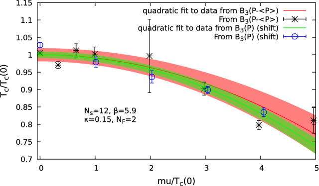
(Ref. [105]) The transition temperature from complex Langevin simulations at heavy pion masses ( GeV with two flavor Wilson fermions on an lattice. The transition temperature is determined from the third order Binder cumulant with two different Polyakov loop related observables. The data is then fitted with a quadratic function
In addition to finite temperature studies, complex Langevin simulations are also used to study low or zero temperature QCD. In Refs. [103, 106, 107], the average quark number is studied on lattices with sizes and . The authors found a plateau for as a function of the chemical potential. It is interpreted as the maximum number of zero momentum quarks that can exist at zero temperature. When the chemical potential is increased enough, it excites the lowest non-zero momentum states.
In Ref. [108], the zero temperature transition between hadronic and nuclear matter at a chemical potential of a third of the nucleon mass is searched for but not found. This contradiction to the physical expectation is related to possible issues with the complex Langevin simulations, which faces difficulties at low or zero temperature.
Effective lattice theories
Full lattice QCD simulations for large baryon chemical potentials are out of reach for the moment. However, some insight can be gained from simulations of effective theories on the lattice. Here usually either the fermions and the spatial gauge links are integrated out, yielding a theory only depending on Polyakov loops, which contains the temporal link variables. Or, as the second common option, spatial and temporal gauge links are integrated out, resulting in a theory with hadronic degrees of freedom. The use of effective theories is limited to a specific parameter range, where the reduction of the degrees of freedom holds true. If it is possible to find overlapping parameter ranges between different theories, one can gain insight in a wide range of phenomena.
Heavy quarkonium
Heavy quarkonium refers to states of matter including heavy quarks, most commonly the charm and bottom quark. In heavy ion collisions, and pairs can usually only be created in early stages of the collision due to the required large energy amount. These heavy bound states are then surrounded by the quark–gluon plasma and can either melt due to the high temperatures or survive until freeze-out. In the latter case, a signature for these particles should be visible in the detectors. Since the melting of different particles depends on the state of the quark–gluon plasma, the observation of quarkonium is a useful tool to enhance our knowledge on QCD at very high temperatures. On the other hand it becomes ever clearer that not only the melting but also the possibility of recombination of quarkonium states has to be taken into account. The interaction between the heavy bound states and the surrounding medium is one of the main questions fueling the work on effective theories. A sketch of the different stages a heavy quark pair goes through in a heavy ion collision is shown at the bottom for Fig. 1 from Ref. [19] where a detailed introduction and review of recent developments for heavy quarkonium can be found.
The input from the lattice to the investigation on quarkonium can be twofold. On the one hand, one could consider the calculation of quarkonium correlators and their spectral functions as for example done in Refs. [109, 110]. Since these studies require zero temperature simulations, they are not part of this review.
On the other hand, the lattice simulations of effective field theories are a very helpful tool to investigate the behavior of quarkonium in a quark–gluon plasma. To arrive at an effective field theory, the difference in scales within the quarkonium is exploited. The mass of a heavy quark is much larger than its velocity v within a bound state and, therefore,
| 24 |
and
| 25 |
The reduction of the degrees of freedom by the integration over different scales is sketched in Fig. 14. While full continuum QCD is valid at all scales, the finite volume of the lattice provides an infrared cut off, while the finite lattice spacing cuts off the ultraviolet divergences. To arrive at a non-relativistic version of QCD called NRQCD (Ref. [111]) the hard gluons and heavy quarks are integrated out. The relevant degrees of freedom are the Pauli spinors and soft gluons. This effective theory itself can be treated by a lattice simulation. On the other hand, a perturbative treatment of NRQCD can be applied to integrate out further degrees of freedom down to an energy scale . This leads to potential NRQCD (pNRQCD, Ref. [112]), with ultrasoft gluons and wavefunctions as remaining degrees of freedom. In this framework the in-medium real-time potential can be investigated. Again, it is possible to study pNRQCD on the lattice. To construct the respective Lagrange functions for the various effective field theories, one identifies the relevant degrees of freedom at each energy scale and constructs a general Lagrange function from symmetry considerations. The relevant prefactors of each term, the so-called Wilson coefficients, are determined by matching. The strength of effective field theories lies in the reduced number of degrees of freedom, which makes computations easier. The trade off is the reduced validity range.
Fig. 14.

(Ref. [19]) Overview over the different scales treated in effective field theories on the lattice. In the first step the lattice introduces a UV cut off by the finite lattice volume and an infrared cut off by the finite lattice spacing. In the next step gluons and heavy quarks are integrated out, yielding a non-relativistic version on QCD called NRQCD. The lattice version of NRQCD again has the respective cut offs. Instead on the lattices NRQCD can also be treated perturbatively to integrate out further degrees of freedom down to an energy scale . This leads to potential NRQCD (pNRQCD) with ultrasoft gluons and wavefunctions as remaining degrees of freedom. pNRQCD can then be studied on the lattice by the investigation of non-local Wilson coefficients
An investigation of the validity of the perturbative treatment of effective field theory was done in Ref. [113]. There, lattice QCD calculations of a wide temperature range from 140 MeV up to temperatures of 5814 MeV with (2+1) flavors of highly improved staggered fermions were performed. The evaluation of the static quark–antiquark potential led to the conclusion that effective field theories can be used between (with r the beginning of the separation between quark and antiquark) to describe color screening reliably.
NRQCD: A large effort to use lattice NRQCD to study the behavior of bottemonium in a quark–gluon plasma has been made by the FASTSTUM collaboration in Refs. [114–118]. The authors calculate the spectrum of bottemonium around the crossover temperature, using (2+1) flavors of Wilson clover fermions on anisotropic lattices. The anisotropy of the lattices improves the NRQCD expansion. On the other hand it also leads to heavy pion masses of MeV, if computations are to be kept affordable.
Another recent investigation of both bottomonium and charmonium using NRQCD has been done in Refs. [119, 120]. Here, a lattice configuration of the HOTQCD collaboration with 2+1 highly improved staggered (HISQ) quarks was used. These ensembles have a realistic pion mass of MeV. Reference [120] was able to sort out previous tensions between Ref. [114] and Ref. [119] on the melting temperatures of quarkonium by relating them to different uncertainties in the spectral reconstruction. It was shown that the mass of the ground state for heavy quarkonium reduces when the temperature is increased. However, in Refs. [121, 122], where the same configurations were analyzed, the mass reduction was not observed.
pNRQCD: To investigate not only the ground state, but also the in-medium behavior of excited quarkonium states, one has to turn to pNRQCD. Here the spectral functions are computed by solving the Schrödinger equation with a static potential. The results show a mass reduction for rising temperatures and agree well with lattice NRQCD results, while contradicting the expectation gained from perturbative pNRQCD.
Recent progress with computations in lattice pNRQCD include the determination of the ratio between the and in Ref. [123]. Here a non-perturbative treatment of pNRQCD is employed, based on the derivation of the generalized Gauss law. The derived potential is matched to lattice QCD results from Refs. [130–132]. The calculation of in-medium spectral functions allows for a prediction on the and ratio, which is shown in Fig. 15. It is also compared to various results from heavy ion collision experiments as well as results from the statistical model of hadronization (Ref. [128]).
Fig. 15.
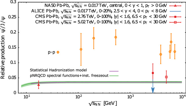
(Ref. [19, 123]) The ratio between and from various heavy ion collision experiments: the NA50 (Ref. [124]), ALICE (Ref. [125]) and CMS (Refs. [126, 127]). The orange points show the pp baseline form Refs. [128, 129]. The purple line comes from the statistical model of hadronization from Ref. [128]. The green line is the result from a computation based on pNRQCD spectral functions combined with an instantaneous freeze-out scenario
Columbia plot
As discussed before, for zero chemical potential and physical quark masses, the QCD transition is a crossover. However, this changes when the quark masses are varied. The type of the transition between hadronic matter and the quark–gluon plasma, called the QCD transition, depends on the quark masses. This is illustrated in the Columbia plot for 2+1 quark flavors (Fig. 16). The upper right corner, where quark masses are infinite, is the pure SU(3) gauge limit with static quarks and exhibits a first order phase transition. Finite quark masses break the Z(3) center symmetry of the zero mass limit explicitly, which weakens the phase transition until it becomes second order in the Z(2) line bordering the upper right corner of the Columbia plot.
Fig. 16.

Schematic of two different, possible scenarios for the Columbia plot. It shows the dependence of the transition between hadronic matter and the quark–gluon plasma on the quark masses
In the limit of vanishing quark masses, corresponding to the lower left corner of the Columbia plot, again a first order transition is expected for three flavors in the chiral limit, where . Finite quark masses break the chiral symmetry and weaken the transition until it becomes of second order. This yields another Z(2) line delimiting this corner. However, the case on the left border, for vanishing light quark masses, is still under investigation. Another possible scenario is that the first order region could extend all the way up to the limit or hit the line at a finite strange quark mass, as shown in Fig. 16. The two scenarios are connected to the possible symmetry reforestation at the transition temperature (Refs. [133, 134]) and are shown in Fig. 16.
The computation of the Z(2) lines, especially in the lower left corner, are numerically very challenging. Smaller quark mass, as well as critical slowing down near a phase transition, increases the computational cost. At the same time, small quark masses increase the taste breaking artifacts for the computationally relatively cheap staggered quarks, making a continuum extrapolation even more difficult. Also, scans in temperature, volume and quark masses are required to determine type and position of the transition. Due to these challenges, the only continuum extrapolated point in the Columbia plot up to now is the physical point (Refs. [1–6]).
To overcome the computational challenges faced when directly investigating the parameter space of the Columbia plot, additional extrapolation directions are used. Simulations at imaginary chemical potential can enlarge the first order region and help to determine it at by limiting the search region. Similarly, simulations at variable , even non-integer ones, have been applied.
Lower left corner
One common direction of investigation is along the diagonal of the Columbia plot. However, the first order region has only been found on lattices with unimproved staggered (Refs. [135, 136]) or O(a)-improved Wilson [137] fermions. For finer lattices or with further improved actions, the phase transition remains elusive (Ref. [138]).
A direct investigation along the border only yielded results for lattices with unimproved staggered or Wilson quarks (Refs. [44, 139, 140]).
A recent investigation of -flavor QCD with small quark masses is reported in Ref. [141]. It studies the Polyakov loop expectation value and the heavy quark free energy
| 26 |
with on lattices. The analysis is done for several volumes to reach the limit . The results for the Polyakov loop and its derivative are shown in Fig. 17. It is found that the scaling behavior is consistent with the scaling behavior for energy-like observables in the 3-d, O(N) universality classes. The authors observe a singular behavior of the quark mass derivatives of and . In the chiral limit the divergence is consistent with the 3-d, O(2) universality class.
Fig. 17.

(Ref. [141]) Top: The temperature dependence of the Polyakov loop . Bottom: The derivative of the Polyakov loop as a function of the scaling varibale with and being non-universal constants
Previously, scaling studies have been carried out in Ref. [142, 143]. Here the transition temperature in the chiral limit and the magnetization
| 27 |
and its derivative, the chiral susceptibility
| 28 |
were determined from lattices with and 12 using the HISQ action. The pion mass was lowered down to MeV and an O(4) scaling ansatz was used to extrapolate to the chiral limit. The final result for the transition temperature in the chiral limit determined from different analyses is given as
| 29 |
The dependence of the chiral susceptibility on the quark masses is shown in the top of Fig. 18. It was determined on an lattice. The spatial extent of the lattice is increased with decreasing light quark mass . It is for or 27, for and for or 160. The dependence on the volume for fixed is shown on the bottom for Fig. 18.
Fig. 18.

(Ref. [142]) Top: The quark mass dependence of the chiral susceptibility as defined in Eq. (28). Bottom: The volume dependence of the chiral susceptibility as defined in Eq. (28)
A further study of the chiral limit is done in Ref. [144]. Here again pion masses down to MeV are used. Lattice spacings of fm 0.08 fm and 0.06 fm correspond to and 16. The authors investigate the dependence of the Dirac eigenvalue spectrum and the axial anomaly on the quark masses. For the chiral condensate they find that while there is a clear dependence on the quark masses and lattice spacing, the volume dependence is small. This is illustrated in Fig. 19.
Fig. 19.

(Ref. [144]) Top: The quark mass dependence of the chiral condensate for different lattice spacings. Bottom: The volume dependence of the chiral condensate for different lattice spacings at MeV
Reference [145] investigates the Columbia plot for the case with improved Wilson quarks and the Iwasaki gauge action up to . It uses multiensemble reweighting to determine the minimum of the kurtosis. The change in this minimum as a function of is then studied for different volumes. The point where it agrees for several volumes defines the critical value. A sketch of this so-called kurtosis intersection analysis is shown in Fig. 20. The results for this analysis for five different values of and the scaling of the maximal chiral susceptibility are shown in Fig. 21. The authors conclude that the Z(2) line in the Columbia plot for the case (along the diagonal) is located at a pion mass MeV.
Fig. 20.

(Ref. [145]) Sketch of the kurtosis intersection analysis. The minimum of the kurtosis is determined from multiensemble reweighting and then fit for different volumes. The intersection is taken to be the value for the critical endpoint, as there should be no volume scaling
Fig. 21.

(Ref. [145]) The scaling exponent of the maximum susceptibility with the volume: . The results are shown for and 12 with connecting lines. The green horizontal line shows the expectation for Z(2)-scaling. The shaded areas show the results for the critical from the kurtosis intersection analysis
Imaginary chemical potential
One way to enlarge the first order region of the Columbia plot, at least on coarse lattices, is the introduction of an imaginary chemical potential. As discussed in Sect. 3.2 there is no sign problem in QCD in the case of a purely imaginary chemical potential. A sketch of this 3-d Columbia plot is shown in Fig. 22. When adding the chemical potential axis to the Columbia plot, its curvature at is negative. This increases, therefore, the first order region for imaginary chemical potential and decreases it for real . These investigations have been done both with unimproved Wilson (Ref. [146]) and staggered (Refs. [147, 148]) fermions on lattices.
Fig. 22.

(Ref. [133]) Sketch of the 3-d Columbia plot with added chemical potential
Variable
Another way to increase the strength of the phase transition, and therefore helping with the investigation of the Columbia plot, is to increase the number of flavors . Reference [149] studies the Columbia plot with four staggered quarks and the Wilson plaquette action. The choice of has the added benefit that no rooting is required. Simulations were performed for , 6, 8 and 10 for several spatial lattice extensions. Figure 23 shows the difference between the critical pion mass for four or three staggered quarks. The increased number of flavors increases the pion mass, so that simulations on lattices with larger temporal extent are possible.
Fig. 23.
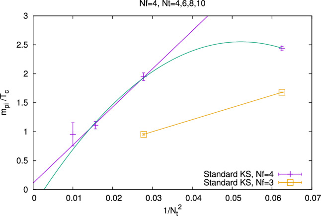
(Ref. [149]) The value of the critical pion mass for four or three staggered quarks, for different values of . For four flavors the critical mass is larger, allowing for finer lattices
To get a smooth transition between the integer number of flavors, it is even possible to consider non-integer powers of the quark determinant (Ref. [139]). This allows for a smooth interpolation in . Since in the chiral limit the transition is of second order for and of first order for there has to be a tricritical scaling area, with a critical point at in between. Reference [139] presents results on lattices for , 2.6, 2.4, 2.2 and 2.1. The dependence of the critical mass for a Z(2) scaling is expected to follow
| 30 |
The results are shown in the top of Fig. 24. The rescaled mass is shown in the bottom of Fig. 24. A linear function was fitted to the rescaled mass to determine C and .
Fig. 24.
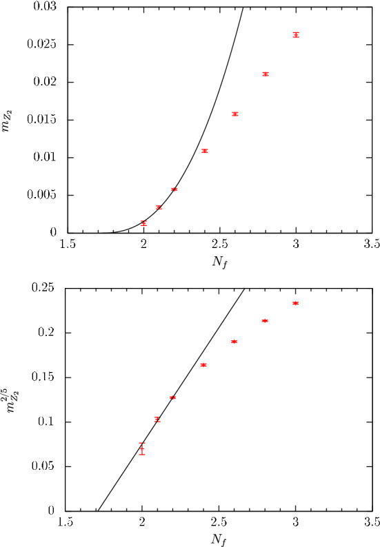
(Ref. [139]) Top: The critical mass as a function of the number of flavor. The black line is the rescaled version of the fit done to the rescaled mass below. Bottom: The rescaled critical mass as a function of the number of flavors. Also we show a linear fit to the data
Overview—lower left corner
The investigation of the Columbia plot remains a challenge for lattice QCD. For the determination of the second order line in the lower left corner (see Fig. 16) several results are available on finite lattices; however, there is no clear solution for the continuum limit. Figure 25 shows an overview over the results for different fermion types. For this plot, some conversions were necessary. Some values were converted to MeV using the value for the critical temperature from Ref. [150] MeV for coarse lattices and staggered quarks. Upper bounds are denoted by zero with the error bar showing the bound. Values given without any error are assumed to have 50% relative error. The color of the points denotes the fermion type used in the simulations. Red stands for unimproved staggered, orange for improved staggered, green for unimproved Wilson and blue for improved Wilson quarks. The largest number of results is available for the three-flavor case. Here both Wilson and staggered quarks show a shrinking value when the lattices become finer. The same trend can be observed for staggered quarks with . For both two and three flavors, staggered quarks show smaller values than Wilson quarks. Also for staggered quarks an improvement of the quark formulation reduces the value for the critical pion mass. Assuming that all quark formulations agree in the continuum, which they should, it seems that still a large amount of computational power is needed to settle the shape of the lower left corner of the Columbia plot. Investigating this region becomes especially challenging since both staggered and Wilson quarks suffer from large lattice artifacts when the quark masses become small (Ref. [151]).
Fig. 25.

Overview over different available results for the critical pion mass in the Columbia plot for , 3 and 4. Values are from Refs. [135–137, 145, 149, 150, 152–156]. The color of the points denotes the fermion type used in the simulations. Red stands for unimproved staggered, orange for improved staggered, green for unimproved Wilson and blue for improved Wilson quarks. Upper bounds are denoted by zero with the error bar showing the bound. Values given without any error are denoted with 50% relative error. Some values were converted to MeV using the value for the critical temperature from Ref. [150] MeV. Similar values for the same have been shifted lightly for more clarity
Upper right corner
Recent progress on the determination of the upper right corner of the Columbia plot (see Fig. 16) was reported in Ref. [157]. The authors determine the critical pion mass for the flavor case. This corresponds to the upper border of the Columbia plot. The lattice setup consisted of two dynamical, degenerate Wilson fermions on lattices with 8 and 10. These values correspond to lattice spacings between 0.07 fm and 0.12 fm. The results for the critical pion masses for all three lattices are shown in the bottom of Fig. 26. While a precise continuum limit is not possible from these three lattices alone, the authors estimate a continuum value of GeV with an error of about 20%. In addition to the critical pion mass, also the critical hopping parameter has been determined. It appears in the fermion matrix for the Wilson quark action as
| 31 |
and controls the bare quark mass by
| 32 |
These results do not agree with those previously computed in Ref. [158]. Here reweighting from quenched QCD has been used to investigate the end-line in 2+1 flavor QCD. For the and case, the results differ by about 50%. Since the same lattice action has been used in the two cases, the discrepancy is most likely related to the different methods and not to the cut off effects. Reference [158] describes finite-volume effects and effects related to the hopping parameter expansion, which seems to shift the results in the direction of Ref. [157].
Fig. 26.

(Ref. [157]) Top: The critical value for the hopping parameter (see Eqs. (32) and (31)) as a function of the lattice spacing. Bottom: Value of the critical pion mass as a function of the lattice spacing
Magnetic fields
When dealing with heavy ion collision experiments, in addition to a finite chemical potential, also the effects of magnetic fields have to be considered (Refs. [159–161]). From zero temperature lattice QCD studies with staggered fermions (Refs. [162–164]) the so-called magnetic catalysis is found. It describes that the chiral condensate, which is an order parameter of the QCD chiral transition, increases with the strength of the magnetic field. From this it was derived that also the transition temperature increases with the magnetic field strength.
A recent study (Ref. [165]) investigated the chiral phase structure of three-flavor QCD with a magnetic field on lattices with four different volumes between and . It uses a Wilson plaquette action with staggered fermions and pion masses of MeV and two values of finite magnetic field strengths. The authors find a strengthening in the transition, which turns to first order when a magnetic field is added. The results for the chiral condensate for different magnetic field strengths and lattice volumes are shown in Fig. 27. The first order nature is derived both from the volume scaling and from metastable states of the chiral condensate in the simulation stream. We also see an increase in the transition temperature with the magnetic field strength.
Fig. 27.

(Ref. [165]) Top: The chiral condensate on a lattice for different magnetic field strengths . Bottom: The chiral condensate for different volumes on lattices with temporal extent at a magnetic field strength of
On the other hand, Refs. [166–171] find a decreasing transition temperature with growing magnetic fields. Here continuum extrapolations or improved actions were employed. It is assumed that the discrepancy is related to discretization artifacts (Ref. [165]). The decreasing of the transition temperature and the chiral condensate is called inverse magnetic catalysis. Most recently, Ref. [171] used the HISQ quark action to study the effects of magnetic fields on a lattice. One could observe the inverse magnetic catalysis even on a finite lattice.
To get a qualitative understanding of the processes leading to a magnetic catalysis or inverse magnetic catalysis, many model studies have been performed (Refs. [163, 172–183]). Lattice studies with heavy pion masses (Refs. [184, 185]) hint toward an explanation for the inverse magnetic catalysis unrelated to the decreasing of the chiral condensate, but related to the quark masses.
Reference [184] uses 2+1 flavors of stout smeared staggered quarks on lattices. One uses pion masses up to MeV and investigates the transition temperature as a function of the magnetic field strength. The transition temperature is determined both from the chiral condensate and the Polyakov loop leading to similar results. The chiral condensate for different strengths of the magnetic field and different pion masses is shown in Figs. 28 and 29. One finds that, while the decrease of the transition temperature is present for all pion masses, the decrease of the chiral condensate, however, is not observable for the highest pion masses. This strengthens the idea that the inverse magnetic catalysis, the decrease of the chiral condensate, is not directly related to the transition temperature. The authors suggest that the decrease of the transition temperature might be a deconfinement catalysis (Ref. [186]).
Fig. 28.

(Ref. [184]) The chiral susceptibility for different strengths of the magnetic field and different pion masses. Simulations were done with stout smeared staggered fermions on lattices. One can observe a decreasing peak position and therefore transition temperature for all pion masses
Fig. 29.
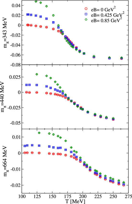
(Ref. [184]) The chiral condensate for different strengths of the magnetic field and different pion masses. Simulations were done with stout smeared staggered fermions on lattices. One can observe that, while for the lightest pion mass the condensate decreases for a stronger magnetic field, it increases for the highest pion mass
Reference [185] determines the transition point in the quark mass between magnetic catalysis and inverse catalysis further. One uses the three stout smeared staggered fermions with physical strange and variable light quark masses. The finite temperature and magnetic field simulations are performed on a lattices. In addition, four different zero temperature lattice simulations without a magnetic field are needed. To determine the mass on the border between magnetic catalysis and inverse magnetic catalysis one looks at the difference between the chiral condensate introduced by a magnetic field defined as
| 33 |
| 34 |
for at the pseudo-critical transition temperature :
| 35 |
A sign change in then determines the value of since for the chiral condensate increases compared to the case without magnetic field while it decreases when . is shown in the top of Fig. 30, indicating . This corresponds to a pion mass of MeV. In addition also the Polyakov loop
| 36 |
from which the ratio
| 37 |
is defined, is investigated. Its behavior around is shown in the top of Fig. 30.
Fig. 30.

(Ref. [185]) Top: The dependence of the chiral condensate defined in Eq. (35) as a function of the pion mass in a magnetic field of GeV. The green line separates the area of the inverse magnetic catalysis (IMC) from the area of the magnetic catalysis (MC) Bottom: The Polyakov loop ratio as defined in Eq. (37) as a function of the magnetic field close to the turning point between inverse magnetic catalysis and magnetic catalysis
The connections between the transition temperature, the quark masses and the chiral condensate in a magnetic field are further investigated in Ref. [164] for zero temperature. The authors connect the chiral condensate and the pion mass by the Gell-Mann–Oakes–Renner relation (Ref. [187]) for two flavors,
| 38 |
and its extension to the three-flavor case (Ref. [188]) with an additional strange quark,
| 39 |
They use a -flavor HISQ quark action on a lattice. The results for the light quark condensate, defined as
| 40 |
are shown in Fig. 31. They find that the Gell-Mann–Oakes–Renner relation for two flavors (Eq. (38)) has only corrections of about 6% when a magnetic field up to is introduced. This illuminates the connection between the reduction of the transition temperature and the pion mass. For the three-flavor case the corrections to the Gell-Mann–Oakes–Renner relation (Eq. (39)) are much larger, namely up to 56%. Another recent investigation of the magnetic catalysis and the inverse magnetic catalysis can be found in Ref. [189]; that study uses the Dyson–Schwinger equations instead of lattice QCD.
Fig. 31.

(Ref. [164]) Top: Ratio between the renormalized up quark and the down quark condensate as a function of eB. Bottom: Ratio between the renormalized up quark and the down quark condensate as a function of
If one wants to match the conditions in heavy ion collisions in addition to the magnetic field a chemical potential should be considered. This causes the above discussed sign problem to reappear. Reference [190], which studies the effect of a magnetic field and a finite baryon density with analytic continuation from imaginary , finds that the inverse magnetic catalysis becomes slightly stronger with increased chemical potential.
Conclusion
The investigation of the QCD phase diagram, especially in relation to heavy ion collision experiments, remains a lively topic for lattice QCD calculations. With newly published results from LHC and RHIC as well as upcoming data from facilities like NICA, CBM and PARC-HI, a better understanding of the QCD phase diagram, including various different influences that duplicate the situation in the colliders as well as possible, is needed.
After the introduction (Sect. 1) and the brief description of the stages of a heavy ion collision experiment (Sect. 2), this review started with the discussion of lattice QCD results at low, finite density (Sect. 3). Accessing the phase diagram with a finite chemical potential is hindered by the infamous sign problem (Sect. 3.1). This is the reason why, for now, continuum extrapolated, physical results are only available as extrapolations (Sect. 3.2). Because the QCD phase transition is an analytic crossover at , one can describe observables with an analytic function that is extrapolated to . There are two techniques for this kind of extrapolation which are commonly used. One can gain information on the dependence of the system either from calculating expansion coefficients from lattice simulations at zero chemical potential (Taylor method) or by describing simulation results at imaginary chemical potential with various functions. The two methods are by now agreeing well on various results. New publications include higher order coefficients on the Taylor expansion of the transition temperature, higher order cumulants of the baryon number distribution, used to compare to heavy ion collision experiments, and higher order cumulants of the baryon number distribution, which are used to compare to heavy ion collision experiments. In addition the possibility to find the QCD critical endpoint is under further investigation. As regards this issue the development of new observables and techniques is necessary.
One method that is getting relatively close to direct lattice simulations at finite density involves complex Langevin simulations (Sect. 3.3). These simulations are based on an evolution in a fictitious Langevin time to generate configurations with a complex measure. Here results are now available for different actions (both fermion and gauge). First comparisons to results from the Taylor expansion method are promising. However, for now results are only available with heavier than physical quark masses and on relatively small lattices.
Another way to access finite density QCD is by effective field theories (Sect. 4), which also can be simulated on the lattice. This review focused on the results for heavy quarkonium (Sect. 4.1). The separation of scales in heavy quark bound states is used to integrate out various degrees of freedom. Lattice simulation can then employ NRQCD or pNRQCD to gain information of heavy quarkonium immersed in the quark–gluon plasma.
Leaving the topic of finite density, also zero density simulations show fascinating progress. By now there are a lot of results on the investigation of the Columbia plot (Sect. 5). The Columbia plot summarizes the dependence of the type of the QCD transition (crossover, first or second order phase transition) on the lighter than physical quark masses. The lower left corner (Sect. 5.1) poses a special computational challenge due to the light quark masses. Therefore, various techniques are employed to gain access to the first order region located there and its critical boundary (Sect. 5.2 and Sect. 5.3). For the case of three degenerate light quarks, results are now available on up to lattices with improved Wilson quarks. However, the continuum extrapolation cannot be carried out yet. This review is therefore restricted to an overview (Sect. 5.4) of the available results for different discretizations. Also the upper right corner of the Columbia plot has been investigated recently (Sect. 5.5). Here the current estimate for the critical pion mass in the continuum is GeV with an error of about 20%.
Finally this review discusses recent results on the influence of a magnetic field (Sect. 6). Like the inclusion of a chemical potential, these effects are relevant for heavy ion collision experiments. An important topic is the distinction between the magnetic catalysis and inverse catalysis which has been related to the light quark masses. Here the lattice results are not in agreement with the common expectation from perturbation theory.
Investigating the QCD phase diagram is a fascinating topic from a purely theoretical point of view. However, many recent results in finite temperature lattice QCD are linked to heavy ion collision experiments. The experimental progress on the quark–gluon plasma allows one on the one hand to confirm the theoretical predictions made by QCD. On the other hand, the computations from lattice QCD are needed by experiments to understand the observations made by the detectors and link them to different stages of collision. This can be done either directly by lattice QCD or through different models or effective theories. In any case the continuation of the experimental heavy ion collision programs will provide interesting checks and challenges for finite temperature lattice QCD calculations.
Acknowledgements
The author thanks Lukas Varnhorst for proofreading and discussion. The project leading to this publication has received funding from Excellence Initiative of Aix-Marseille University - A*MIDEX, a French “Investissements d’Avenir” programme, AMX-18-ACE-005.
Data Availability Statement
This manuscript has no associated data or the data will not be deposited. [Authors’ comment: As a review this manuscript does not have original data. Some data may be found accompanying the referenced work.]
References
- 1.Aoki Y, Endrodi G, Fodor Z, Katz SD, Szabo KK. Nature. 2006;443:675. doi: 10.1038/nature05120. [DOI] [PubMed] [Google Scholar]
- 2.Aoki Y, Fodor Z, Katz S, Szabo K. Phys. Lett. B. 2006;643:46. doi: 10.1016/j.physletb.2006.10.021. [DOI] [Google Scholar]
- 3.Aoki Y, Borsanyi S, Durr S, Fodor Z, Katz SD, Krieg S, Szabo KK. JHEP. 2009;06:088. doi: 10.1088/1126-6708/2009/06/088. [DOI] [Google Scholar]
- 4.S. Borsanyi, Z. Fodor, C. Hoelbling, S.D. Katz, S. Krieg, C. Ratti, K.K. Szabo (Wuppertal-Budapest), JHEP 09, 073 (2010), arXiv:1005.3508
- 5.Bhattacharya T, et al. Phys. Rev. Lett. 2014;113:082001. doi: 10.1103/PhysRevLett.113.082001. [DOI] [PubMed] [Google Scholar]
- 6.Bazavov A, et al. Phys. Rev. D. 2012;85:054503. doi: 10.1103/PhysRevD.85.054503. [DOI] [Google Scholar]
- 7.Barbour IM, Morrison SE, Klepfish EG, Kogut JB, Lombardo MP. Nucl. Phys. B Proc. Suppl. 1998;60:220. doi: 10.1016/S0920-5632(97)00484-2. [DOI] [Google Scholar]
- 8.Fodor Z, Katz SD. Phys. Lett. B. 2002;534:87. doi: 10.1016/S0370-2693(02)01583-6. [DOI] [Google Scholar]
- 9.Fodor Z, Katz SD. JHEP. 2002;03:014. doi: 10.1088/1126-6708/2002/03/014. [DOI] [Google Scholar]
- 10.Csikor F, Egri G, Fodor Z, Katz S, Szabo K, Toth A. Nucl. Phys. B Proc. Suppl. 2003;119:547. doi: 10.1016/S0920-5632(03)80453-X. [DOI] [Google Scholar]
- 11.Fodor Z, Katz SD, Schmidt C. JHEP. 2007;03:121. doi: 10.1088/1126-6708/2007/03/121. [DOI] [Google Scholar]
- 12.Alexandru A, Gattringer C, Schadler HP, Splittorff K, Verbaarschot J. Phys. Rev. D. 2015;91:074501. doi: 10.1103/PhysRevD.91.074501. [DOI] [Google Scholar]
- 13.Alexandru A, Faber M, Horvath I, Liu KF. Phys. Rev. D. 2005;72:114513. doi: 10.1103/PhysRevD.72.114513. [DOI] [Google Scholar]
- 14.S. Kratochvila, P. de Forcrand, PoS LAT2005, 167 (2006), arXiv:hep-lat/0509143
- 15.Ejiri S. Phys. Rev. D. 2008;78:074507. doi: 10.1103/PhysRevD.78.074507. [DOI] [Google Scholar]
- 16.C. Gattringer, PoS LATTICE2013, 002 (2014), arXiv:1401.7788
- 17.L. Scorzato, PoS LATTICE2015, 016 (2016), arXiv:1512.08039
- 18.Alexandru A, Basar G, Bedaque P. Phys. Rev. D. 2016;93:014504. doi: 10.1103/PhysRevD.93.014504. [DOI] [Google Scholar]
- 19.Rothkopf A. Phys. Rept. 2020;858:1. doi: 10.1016/j.physrep.2020.02.006. [DOI] [Google Scholar]
- 20.Gelis F, Iancu E, Jalilian-Marian J, Venugopalan R. Ann. Rev. Nucl. Part. Sci. 2010;60:463. doi: 10.1146/annurev.nucl.010909.083629. [DOI] [Google Scholar]
- 21.Gelis F. Int. J. Mod. Phys. A. 2013;28:1330001. doi: 10.1142/S0217751X13300019. [DOI] [Google Scholar]
- 22.Rischke DH. Prog. Part. Nucl. Phys. 2004;52:197. doi: 10.1016/j.ppnp.2003.09.002. [DOI] [Google Scholar]
- 23.Hasenfratz P, Karsch F. Phys. Lett. B. 1983;125:308. doi: 10.1016/0370-2693(83)91290-X. [DOI] [Google Scholar]
- 24.Allton CR, Ejiri S, Hands SJ, Kaczmarek O, Karsch F, Laermann E, Schmidt C, Scorzato L. Phys. Rev. D. 2002;66:074507. doi: 10.1103/PhysRevD.66.074507. [DOI] [Google Scholar]
- 25.Allton CR, Doring M, Ejiri S, Hands SJ, Kaczmarek O, Karsch F, Laermann E, Redlich K. Phys. Rev. D. 2005;71:054508. doi: 10.1103/PhysRevD.71.054508. [DOI] [Google Scholar]
- 26.Gavai RV, Gupta S. Phys. Rev. D. 2008;78:114503. doi: 10.1103/PhysRevD.78.114503. [DOI] [Google Scholar]
- 27.S. Basak et al. (MILC), PoS LATTICE2008, 171 (2008), arXiv:0910.0276
- 28.Kaczmarek O, Karsch F, Laermann E, Miao C, Mukherjee S, Petreczky P, Schmidt C, Soeldner W, Unger W. Phys. Rev. D. 2011;83:014504. doi: 10.1103/PhysRevD.83.014504. [DOI] [Google Scholar]
- 29.Seiler E, Sexty D, Stamatescu IO. Phys. Lett. B. 2013;723:213. doi: 10.1016/j.physletb.2013.04.062. [DOI] [Google Scholar]
- 30.Sexty D. Phys. Lett. B. 2014;729:108. doi: 10.1016/j.physletb.2014.01.019. [DOI] [Google Scholar]
- 31.Borsanyi S, Fodor Z, Katz SD, Krieg S, Ratti C, Szabo K. JHEP. 2012;01:138. doi: 10.1007/JHEP01(2012)138. [DOI] [Google Scholar]
- 32.Borsanyi S, Endrodi G, Fodor Z, Katz S, Krieg S, Ratti C, Szabo K. JHEP. 2012;08:053. doi: 10.1007/JHEP08(2012)053. [DOI] [Google Scholar]
- 33.Bellwied R, Borsanyi S, Fodor Z, Katz SD, Pasztor A, Ratti C, Szabo KK. Phys. Rev. D. 2015;92:114505. doi: 10.1103/PhysRevD.92.114505. [DOI] [Google Scholar]
- 34.Ding HT, Mukherjee S, Ohno H, Petreczky P, Schadler HP. Phys. Rev. D. 2015;92:074043. doi: 10.1103/PhysRevD.92.074043. [DOI] [Google Scholar]
- 35.Bazavov A, et al. Phys. Rev. D. 2017;95:054504. doi: 10.1103/PhysRevD.95.054504. [DOI] [Google Scholar]
- 36.A. Bazavov et al. (HotQCD), Phys. Lett. B795, 15 (2019), arXiv:1812.08235
- 37.Bazavov A, et al. Phys. Rev. D. 2020;101:074502. doi: 10.1103/PhysRevD.101.074502. [DOI] [Google Scholar]
- 38.Bonati C, D’Elia M, Negro F, Sanfilippo F, Zambello K. Phys. Rev. D. 2018;98:054510. doi: 10.1103/PhysRevD.98.054510. [DOI] [Google Scholar]
- 39.Endrodi G, Fodor Z, Katz SD, Szabo KK. JHEP. 2011;04:001. doi: 10.1007/JHEP04(2011)001. [DOI] [Google Scholar]
- 40.de Forcrand P, Philipsen O. Nucl. Phys. B. 2002;642:290. doi: 10.1016/S0550-3213(02)00626-0. [DOI] [Google Scholar]
- 41.D’Elia M, Lombardo MP. Phys. Rev. D. 2003;67:014505. doi: 10.1103/PhysRevD.67.014505. [DOI] [Google Scholar]
- 42.D’Elia M, Sanfilippo F. Phys. Rev. D. 2009;80:014502. doi: 10.1103/PhysRevD.80.014502. [DOI] [Google Scholar]
- 43.Cea P, Cosmai L, Papa A. Phys. Rev. D. 2014;89:074512. doi: 10.1103/PhysRevD.89.074512. [DOI] [Google Scholar]
- 44.Bonati C, de Forcrand P, D’Elia M, Philipsen O, Sanfilippo F. Phys. Rev. D. 2014;90:074030. doi: 10.1103/PhysRevD.90.074030. [DOI] [Google Scholar]
- 45.Cea P, Cosmai L, Papa A. Phys. Rev. D. 2016;93:014507. doi: 10.1103/PhysRevD.93.014507. [DOI] [Google Scholar]
- 46.Bonati C, D’Elia M, Mariti M, Mesiti M, Negro F, Sanfilippo F. Phys. Rev. D. 2015;92:054503. doi: 10.1103/PhysRevD.92.054503. [DOI] [Google Scholar]
- 47.Bellwied R, Borsanyi S, Fodor Z, Guenther J, Katz SD, Ratti C, Szabo KK. Phys. Lett. B. 2015;751:559. doi: 10.1016/j.physletb.2015.11.011. [DOI] [Google Scholar]
- 48.D’Elia M, Gagliardi G, Sanfilippo F. Phys. Rev. D. 2017;95:094503. doi: 10.1103/PhysRevD.95.094503. [DOI] [Google Scholar]
- 49.Guenther JN, Bellwied R, Borsanyi S, Fodor Z, Katz SD, Pasztor A, Ratti C, Szabó KK. Nucl. Phys. A. 2017;967:720. doi: 10.1016/j.nuclphysa.2017.05.044. [DOI] [Google Scholar]
- 50.Alba P, et al. Phys. Rev. D. 2017;96:034517. doi: 10.1103/PhysRevD.96.034517. [DOI] [Google Scholar]
- 51.Vovchenko V, Pasztor A, Fodor Z, Katz SD, Stoecker H. Phys. Lett. B. 2017;775:71. doi: 10.1016/j.physletb.2017.10.042. [DOI] [Google Scholar]
- 52.S. Borsanyi, Z. Fodor, J.N. Guenther, S.K. Katz, K.K. Szabo, A. Pasztor, I. Portillo, C. Ratti (2018), arXiv:1805.04445
- 53.S. Borsanyi, Z. Fodor, J.N. Guenther, R. Kara, S.D. Katz, P. Parotto, A. Pasztor, C. Ratti, K.K. Szabo (2020), arXiv:2002.02821 [DOI] [PubMed]
- 54.R. Bellwied, S. Borsányi, Z. Fodor, J. Günther, S.D. Katz, K.K. Szabó, C. Ratti, A. Pasztor, PoS ICHEP2016, 369 (2016)
- 55.A. Pásztor, Z. Szép, G. Markó (2020), arXiv:2010.00394
- 56.P. Steinbrecher (HotQCD), Nucl. Phys. A 982, 847 (2019), arXiv:1807.05607
- 57.Isserstedt P, Buballa M, Fischer CS, Gunkel PJ. Phys. Rev. D. 2019;100:074011. doi: 10.1103/PhysRevD.100.074011. [DOI] [Google Scholar]
- 58.Andronic A, Braun-Munzinger P, Stachel J. Nucl. Phys. A. 2006;772:167. doi: 10.1016/j.nuclphysa.2006.03.012. [DOI] [Google Scholar]
- 59.Becattini F, Bleicher M, Kollegger T, Schuster T, Steinheimer J, Stock R. Phys. Rev. Lett. 2013;111:082302. doi: 10.1103/PhysRevLett.111.082302. [DOI] [PubMed] [Google Scholar]
- 60.P. Alba, W. Alberico, R. Bellwied, M. Bluhm, V. Mantovani Sarti, M. Nahrgang, C. Ratti, Phys. Lett. B738, 305 (2014), arXiv:1403.4903
- 61.Vovchenko V, Begun VV, Gorenstein MI. Phys. Rev. C. 2016;93:064906. doi: 10.1103/PhysRevC.93.064906. [DOI] [Google Scholar]
- 62.L. Adamczyk et al. (STAR), Phys. Rev. C96, 044904 (2017), arXiv:1701.07065
- 63.Y. Hatta, M. Stephanov, Phys. Rev. Lett. 91, 102003 (2003), [Erratum: Phys.Rev.Lett. 91, 129901 (2003)], arXiv:hep-ph/0302002
- 64.Stephanov M. Phys. Rev. Lett. 2009;102:032301. doi: 10.1103/PhysRevLett.102.032301. [DOI] [PubMed] [Google Scholar]
- 65.Friman B, Karsch F, Redlich K, Skokov V. Eur. Phys. J. C. 2011;71:1694. doi: 10.1140/epjc/s10052-011-1694-2. [DOI] [Google Scholar]
- 66.Halasz AM, Jackson A, Shrock R, Stephanov MA, Verbaarschot J. Phys. Rev. D. 1998;58:096007. doi: 10.1103/PhysRevD.58.096007. [DOI] [Google Scholar]
- 67.Stephanov MA, Rajagopal K, Shuryak EV. Phys. Rev. D. 1999;60:114028. doi: 10.1103/PhysRevD.60.114028. [DOI] [Google Scholar]
- 68.Cheng M, et al. Phys. Rev. D. 2008;77:014511. doi: 10.1103/PhysRevD.77.014511. [DOI] [Google Scholar]
- 69.A. Bazavov et al. (HotQCD) (2017), arXiv:1708.04897
- 70.Karsch F. Central. Eur. J. Phys. 2012;10:1234. [Google Scholar]
- 71.Bazavov A, et al. Phys. Rev. Lett. 2012;109:192302. doi: 10.1103/PhysRevLett.109.192302. [DOI] [PubMed] [Google Scholar]
- 72.Borsanyi S, Fodor Z, Katz SD, Krieg S, Ratti C, Szabo KK. Phys. Rev. Lett. 2013;111:062005. doi: 10.1103/PhysRevLett.111.062005. [DOI] [PubMed] [Google Scholar]
- 73.Borsanyi S, Fodor Z, Katz SD, Krieg S, Ratti C, Szabo KK. Phys. Rev. Lett. 2014;113:052301. doi: 10.1103/PhysRevLett.113.052301. [DOI] [PubMed] [Google Scholar]
- 74.Ratti C. Rept. Prog. Phys. 2018;81:084301. doi: 10.1088/1361-6633/aabb97. [DOI] [PubMed] [Google Scholar]
- 75.J. Adam et al. (STAR) (2020), arXiv:2001.02852
- 76.T. Nonaka (STAR), Measurement of the Sixth-Order Cumulant of Net-Proton Distributions in Au+Au Collisions from the STAR Experiment, in 28th International Conference on Ultrarelativistic Nucleus-Nucleus Collisions (2020), arXiv:2002.12505
- 77.Bellwied R, Borsanyi S, Fodor Z, Guenther JN, Noronha-Hostler J, Parotto P, Pasztor A, Ratti C, Stafford JM. Phys. Rev. D. 2020;101:034506. doi: 10.1103/PhysRevD.101.034506. [DOI] [Google Scholar]
- 78.Begun V, Gorenstein MI, Hauer M, Konchakovski V, Zozulya O. Phys. Rev. C. 2006;74:044903. doi: 10.1103/PhysRevC.74.044903. [DOI] [Google Scholar]
- 79.Kitazawa M, Asakawa M. Phys. Rev. C. 2012;85:021901. doi: 10.1103/PhysRevC.85.021901. [DOI] [Google Scholar]
- 80.M. Kitazawa, M. Asakawa, Phys. Rev. C 86, 024904 (2012), [Erratum: Phys.Rev.C 86, 069902 (2012)], arXiv:1205.3292
- 81.Giordano M, Pásztor A. Phys. Rev. D. 2019;99:114510. doi: 10.1103/PhysRevD.99.114510. [DOI] [Google Scholar]
- 82.Lee T, Yang CN. Phys. Rev. 1952;87:410. doi: 10.1103/PhysRev.87.410. [DOI] [Google Scholar]
- 83.Hasenfratz A, Toussaint D. Nucl. Phys. B. 1992;371:539. doi: 10.1016/0550-3213(92)90247-9. [DOI] [Google Scholar]
- 84.Fodor Z, Katz SD. JHEP. 2004;04:050. doi: 10.1088/1126-6708/2004/04/050. [DOI] [Google Scholar]
- 85.Danzer J, Gattringer C. Phys. Rev. D. 2008;78:114506. doi: 10.1103/PhysRevD.78.114506. [DOI] [Google Scholar]
- 86.Alexandru A, Wenger U. Phys. Rev. D. 2011;83:034502. doi: 10.1103/PhysRevD.83.034502. [DOI] [Google Scholar]
- 87.Giordano M, Kapas K, Katz SD, Nogradi D, Pasztor A. Phys. Rev. D. 2020;101:074511. doi: 10.1103/PhysRevD.101.074511. [DOI] [Google Scholar]
- 88.Giordano M, Kapas K, Katz SD, Nogradi D, Pasztor A. JHEP. 2020;05:088. doi: 10.1007/JHEP05(2020)088. [DOI] [Google Scholar]
- 89.F. Attanasio, B. Jäger, F.P. Ziegler (2020), arXiv:2006.00476
- 90.Ambjorn J, Yang S. Phys. Lett. B. 1985;165:140. doi: 10.1016/0370-2693(85)90708-7. [DOI] [Google Scholar]
- 91.Klauder JR, Petersen WP. J. Stat. Phys. 1985;39:53. doi: 10.1007/BF01007974. [DOI] [Google Scholar]
- 92.Lin HQ, Hirsch JE. Phys. Rev. B. 1986;34:1964. doi: 10.1103/PhysRevB.34.1964. [DOI] [PubMed] [Google Scholar]
- 93.Ambjorn J, Flensburg M, Peterson C. Nucl. Phys. B. 1986;275:375. doi: 10.1016/0550-3213(86)90605-X. [DOI] [Google Scholar]
- 94.Aarts G, Bongiovanni L, Seiler E, Sexty D, Stamatescu IO. Eur. Phys. J. A. 2013;49:89. doi: 10.1140/epja/i2013-13089-4. [DOI] [Google Scholar]
- 95.Berges J, Sexty D. Nucl. Phys. B. 2008;799:306. doi: 10.1016/j.nuclphysb.2008.01.018. [DOI] [Google Scholar]
- 96.Aarts G, James FA, Seiler E, Stamatescu IO. Phys. Lett. B. 2010;687:154. doi: 10.1016/j.physletb.2010.03.012. [DOI] [Google Scholar]
- 97.Attanasio F, Jäger B. Eur. Phys. J. C. 2019;79:16. doi: 10.1140/epjc/s10052-018-6512-7. [DOI] [Google Scholar]
- 98.Nishimura J, Shimasaki S. Phys. Rev. D. 2015;92:011501. doi: 10.1103/PhysRevD.92.011501. [DOI] [Google Scholar]
- 99.G. Aarts, E. Seiler, D. Sexty, I.O. Stamatescu, JHEP 05, 044 (2017), [Erratum: JHEP 01, 128 (2018)], arXiv:1701.02322
- 100.Nagata K, Nishimura J, Shimasaki S. Phys. Rev. D. 2016;94:114515. doi: 10.1103/PhysRevD.94.114515. [DOI] [Google Scholar]
- 101.Nagata K, Nishimura J, Shimasaki S. JHEP. 2018;05:004. doi: 10.1007/JHEP05(2018)004. [DOI] [Google Scholar]
- 102.Scherzer M, Seiler E, Sexty D, Stamatescu IO. Phys. Rev. D. 2019;99:014512. doi: 10.1103/PhysRevD.99.014512. [DOI] [Google Scholar]
- 103.S. Tsutsui, Y. Ito, H. Matsufuru, J. Nishimura, S. Shimasaki, A. Tsuchiya, PoS LATTICE2019, 151 (2019), arXiv:1912.00361
- 104.Sexty D. Phys. Rev. D. 2019;100:074503. doi: 10.1103/PhysRevD.100.074503. [DOI] [Google Scholar]
- 105.Scherzer M, Sexty D, Stamatescu IO. Phys. Rev. D. 2020;102:014515. doi: 10.1103/PhysRevD.102.014515. [DOI] [Google Scholar]
- 106.Y. Ito, H. Matsufuru, J. Nishimura, S. Shimasaki, A. Tsuchiya, S. Tsutsui, PoS LATTICE2018, 146 (2018), arXiv:1811.12688
- 107.Ito Y, Matsufuru H, Namekawa Y, Nishimura J, Shimasaki S, Tsuchiya A, Tsutsui S. JHEP. 2020;10:144. doi: 10.1007/JHEP10(2020)144. [DOI] [Google Scholar]
- 108.Kogut J, Sinclair D. Phys. Rev. D. 2019;100:054512. doi: 10.1103/PhysRevD.100.054512. [DOI] [Google Scholar]
- 109.Karsch F, Laermann E, Petreczky P, Stickan S. Phys. Rev. D. 2003;68:014504. doi: 10.1103/PhysRevD.68.014504. [DOI] [Google Scholar]
- 110.G. Aarts, J.M. Martinez Resco, Nucl. Phys. B 726, 93 (2005), arXiv:hep-lat/0507004
- 111.Caswell W, Lepage G. Phys. Lett. B. 1986;167:437. doi: 10.1016/0370-2693(86)91297-9. [DOI] [Google Scholar]
- 112.Brambilla N, Pineda A, Soto J, Vairo A. Nucl. Phys. B. 2000;566:275. doi: 10.1016/S0550-3213(99)00693-8. [DOI] [Google Scholar]
- 113.A. Bazavov, N. Brambilla, P. Petreczky, A. Vairo, J.H. Weber (TUMQCD), Phys. Rev. D 98, 054511 (2018), arXiv:1804.10600
- 114.Aarts G, Allton C, Harris T, Kim S, Lombardo MP, Ryan SM, Skullerud JI. JHEP. 2014;07:097. doi: 10.1007/JHEP07(2014)097. [DOI] [Google Scholar]
- 115.Aarts G, Allton C, Kim S, Lombardo M, Ryan S, Skullerud JI. JHEP. 2013;12:064. doi: 10.1007/JHEP12(2013)064. [DOI] [Google Scholar]
- 116.Aarts G, Allton C, Kim S, Lombardo MP, Oktay MB, Ryan SM, Sinclair D, Skullerud JI. JHEP. 2013;03:084. doi: 10.1007/JHEP03(2013)084. [DOI] [PubMed] [Google Scholar]
- 117.Aarts G, Allton C, Kim S, Lombardo M, Oktay M, Ryan S, Sinclair D, Skullerud J. JHEP. 2011;11:103. doi: 10.1007/JHEP11(2011)103. [DOI] [PubMed] [Google Scholar]
- 118.Aarts G, Kim S, Lombardo M, Oktay M, Ryan S, Sinclair D, Skullerud JI. Phys. Rev. Lett. 2011;106:061602. doi: 10.1103/PhysRevLett.106.061602. [DOI] [PubMed] [Google Scholar]
- 119.Kim S, Petreczky P, Rothkopf A. Phys. Rev. D. 2015;91:054511. doi: 10.1103/PhysRevD.91.054511. [DOI] [Google Scholar]
- 120.Kim S, Petreczky P, Rothkopf A. JHEP. 2018;11:088. doi: 10.1007/JHEP11(2018)088. [DOI] [Google Scholar]
- 121.Larsen R, Meinel S, Mukherjee S, Petreczky P. Phys. Lett. B. 2020;800:135119. doi: 10.1016/j.physletb.2019.135119. [DOI] [Google Scholar]
- 122.Larsen R, Meinel S, Mukherjee S, Petreczky P. Phys. Rev. D. 2019;100:074506. doi: 10.1103/PhysRevD.100.074506. [DOI] [Google Scholar]
- 123.Lafferty D, Rothkopf A. Phys. Rev. D. 2020;101:056010. doi: 10.1103/PhysRevD.101.056010. [DOI] [Google Scholar]
- 124.Alessandro B, et al. NA50. Eur. Phys. J. C. 2007;49:559. doi: 10.1140/epjc/s10052-006-0153-y. [DOI] [Google Scholar]
- 125.J. Adam et al. (ALICE), JHEP 05, 179 (2016), arXiv:1506.08804
- 126.Khachatryan V, et al. CMS. Phys. Rev. Lett. 2014;113:262301. doi: 10.1103/PhysRevLett.113.262301. [DOI] [PubMed] [Google Scholar]
- 127.A.M. Sirunyan et al. (CMS), Phys. Rev. Lett. 118, 162301 (2017), arXiv:1611.01438 [DOI] [PubMed]
- 128.Andronic A, Braun-Munzinger P, Redlich K, Stachel J. Nature. 2018;561:321. doi: 10.1038/s41586-018-0491-6. [DOI] [PubMed] [Google Scholar]
- 129.A. Drees (PHENIX), Nucl. Part. Phys. Proc. 289-290, 417 (2017)
- 130.Burnier Y, Kaczmarek O, Rothkopf A. JHEP. 2015;12:101. doi: 10.1103/PhysRevLett.114.082001. [DOI] [PubMed] [Google Scholar]
- 131.Burnier Y, Kaczmarek O, Rothkopf A. Phys. Rev. Lett. 2015;114:082001. doi: 10.1103/PhysRevLett.114.082001. [DOI] [PubMed] [Google Scholar]
- 132.Bazavov A, et al. MILC. Rev. Mod. Phys. 2010;82:1349. doi: 10.1103/RevModPhys.82.1349. [DOI] [Google Scholar]
- 133.O. Philipsen, PoS LATTICE2019, 273 (2019), arXiv:1912.04827
- 134.Pelissetto A, Vicari E. Phys. Rev. D. 2013;88:105018. doi: 10.1103/PhysRevD.88.105018. [DOI] [Google Scholar]
- 135.Karsch F, Laermann E, Schmidt C. Phys. Lett. B. 2001;520:41. doi: 10.1016/S0370-2693(01)01114-5. [DOI] [Google Scholar]
- 136.de Forcrand P, Philipsen O. Nucl. Phys. B. 2003;673:170. doi: 10.1016/j.nuclphysb.2003.09.005. [DOI] [Google Scholar]
- 137.Jin XY, Kuramashi Y, Nakamura Y, Takeda S, Ukawa A. Phys. Rev. D. 2015;91:014508. doi: 10.1103/PhysRevD.91.014508. [DOI] [Google Scholar]
- 138.Bazavov A, Ding HT, Hegde P, Karsch F, Laermann E, Mukherjee S, Petreczky P, Schmidt C. Phys. Rev. D. 2017;95:074505. doi: 10.1103/PhysRevD.95.074505. [DOI] [PubMed] [Google Scholar]
- 139.Cuteri F, Philipsen O, Sciarra A. Phys. Rev. D. 2018;97:114511. doi: 10.1103/PhysRevD.97.114511. [DOI] [Google Scholar]
- 140.Philipsen O, Pinke C. Phys. Rev. D. 2016;93:114507. doi: 10.1103/PhysRevD.93.114507. [DOI] [Google Scholar]
- 141.D.A. Clarke, O. Kaczmarek, F. Karsch, A. Lahiri, M. Sarkar (2020), arXiv:2008.11678
- 142.Ding H, et al. Phys. Rev. Lett. 2019;123:062002. doi: 10.1103/PhysRevLett.123.062002. [DOI] [PubMed] [Google Scholar]
- 143.H.T. Ding, P. Hegde, O. Kaczmarek, F. Karsch, A. Lahiri, S.T. Li, S. Mukherjee, P. Petreczky (HotQCD), PoS LATTICE2018, 171 (2019), arXiv:1905.11610
- 144.H.T. Ding, S.T. Li, S. Mukherjee, A. Tomiya, X.D. Wang, Y. Zhang (2020), arXiv:2010.14836
- 145.Kuramashi Y, Nakamura Y, Ohno H, Takeda S. Phys. Rev. D. 2020;101:054509. doi: 10.1103/PhysRevD.101.054509. [DOI] [Google Scholar]
- 146.Philipsen O, Pinke C. Phys. Rev. D. 2014;89:094504. doi: 10.1103/PhysRevD.89.094504. [DOI] [Google Scholar]
- 147.de Forcrand P, Philipsen O. Phys. Rev. Lett. 2010;105:152001. doi: 10.1103/PhysRevLett.105.152001. [DOI] [PubMed] [Google Scholar]
- 148.Bonati C, Cossu G, D’Elia M, Sanfilippo F. Phys. Rev. D. 2011;83:054505. doi: 10.1103/PhysRevD.83.054505. [DOI] [Google Scholar]
- 149.P. de Forcrand, M. D’Elia, PoS LATTICE2016, 081 (2017), arXiv:1702.00330
- 150.Karsch F, Laermann E, Peikert A. Nucl. Phys. B. 2001;605:579. doi: 10.1016/S0550-3213(01)00200-0. [DOI] [Google Scholar]
- 151.Iwasaki Y, Kanaya K, Kaya S, Sakai S, Yoshie T. Phys. Rev. D. 1996;54:7010. doi: 10.1103/PhysRevD.54.7010. [DOI] [PubMed] [Google Scholar]
- 152.L. Varnhorst, PoS LATTICE2014, 193 (2015)
- 153.P. de Forcrand, S. Kim, O. Philipsen, PoS LATTICE2007, 178 (2007), arXiv:0711.0262
- 154.Karsch F, Allton C, Ejiri S, Hands S, Kaczmarek O, Laermann E, Schmidt C. Nucl. Phys. B Proc. Suppl. 2004;129:614. doi: 10.1016/S0920-5632(03)02659-8. [DOI] [Google Scholar]
- 155.G. Endrodi, Z. Fodor, S. Katz, K. Szabo, PoS LATTICE2007, 182 (2007), arXiv:0710.0998
- 156.H.T. Ding, A. Bazavov, P. Hegde, F. Karsch, S. Mukherjee, P. Petreczky, PoS LATTICE2011, 191 (2011), arXiv:1111.0185
- 157.F. Cuteri, O. Philipsen, A. Schön, A. Sciarra (2020), arXiv:2009.14033
- 158.S. Ejiri, S. Itagaki, R. Iwami, K. Kanaya, M. Kitazawa, A. Kiyohara, M. Shirogane, T. Umeda (WHOT-QCD), Phys. Rev. D 101, 054505 (2020), arXiv:1912.10500
- 159.Kharzeev DE, McLerran LD, Warringa HJ. Nucl. Phys. A. 2008;803:227. doi: 10.1016/j.nuclphysa.2008.02.298. [DOI] [Google Scholar]
- 160.Skokov V, Illarionov A, Toneev V. Int. J. Mod. Phys. A. 2009;24:5925. doi: 10.1142/S0217751X09047570. [DOI] [Google Scholar]
- 161.Deng WT, Huang XG. Phys. Rev. C. 2012;85:044907. doi: 10.1103/PhysRevC.85.044907. [DOI] [Google Scholar]
- 162.D’Elia M, Mukherjee S, Sanfilippo F. Phys. Rev. D. 2010;82:051501. doi: 10.1103/PhysRevD.82.051501. [DOI] [Google Scholar]
- 163.Shovkovy IA. Mag. Catalysis. 2013;871:13–49. [Google Scholar]
- 164.H.T. Ding, S.T. Li, A. Tomiya, X.D. Wang, Y. Zhang (2020), arXiv:2008.00493
- 165.H.T. Ding, C. Schmidt, A. Tomiya, X.D. Wang (2020), arXiv:2006.13422
- 166.Bali G, Bruckmann F, Endrodi G, Fodor Z, Katz S, Krieg S, Schafer A, Szabo K. JHEP. 2012;02:044. doi: 10.1007/JHEP02(2012)044. [DOI] [Google Scholar]
- 167.Bali G, Bruckmann F, Endrodi G, Fodor Z, Katz S, Schafer A. Phys. Rev. D. 2012;86:071502. doi: 10.1103/PhysRevD.86.071502. [DOI] [Google Scholar]
- 168.Ilgenfritz EM, Muller-Preussker M, Petersson B, Schreiber A. Phys. Rev. D. 2014;89:054512. doi: 10.1103/PhysRevD.89.054512. [DOI] [Google Scholar]
- 169.Bornyakov V, Buividovich P, Cundy N, Kochetkov O, Schäfer A. Phys. Rev. D. 2014;90:034501. doi: 10.1103/PhysRevD.90.034501. [DOI] [Google Scholar]
- 170.Bali G, Bruckmann F, Endrödi G, Katz S, Schäfer A. JHEP. 2014;08:177. doi: 10.1007/JHEP08(2014)177. [DOI] [Google Scholar]
- 171.A. Tomiya, H.T. Ding, X.D. Wang, Y. Zhang, S. Mukherjee, C. Schmidt, PoS LATTICE2018, 163 (2019), arXiv:1904.01276
- 172.D’Elia M, Negro F. Phys. Rev. D. 2011;83:114028. doi: 10.1103/PhysRevD.83.114028. [DOI] [Google Scholar]
- 173.Andersen JO, Naylor WR, Tranberg A. Rev. Mod. Phys. 2016;88:025001. doi: 10.1103/RevModPhys.88.025001. [DOI] [Google Scholar]
- 174.Kojo T, Su N. Phys. Lett. B. 2013;720:192. doi: 10.1016/j.physletb.2013.02.024. [DOI] [Google Scholar]
- 175.Bruckmann F, Endrodi G, Kovacs TG. JHEP. 2013;04:112. doi: 10.1007/JHEP04(2013)112. [DOI] [Google Scholar]
- 176.Fukushima K, Hidaka Y. Phys. Rev. Lett. 2013;110:031601. doi: 10.1103/PhysRevLett.110.031601. [DOI] [PubMed] [Google Scholar]
- 177.Ferreira M, Costa P, Lourenço O, Frederico T, Providência C. Phys. Rev. D. 2014;89:116011. doi: 10.1103/PhysRevD.89.116011. [DOI] [Google Scholar]
- 178.Yu L, Liu H, Huang M. Phys. Rev. D. 2014;90:074009. doi: 10.1103/PhysRevD.90.074009. [DOI] [Google Scholar]
- 179.B. Feng, D. Hou, H.c. Ren, P.p. Wu, Phys. Rev. D 93, 085019 (2016), arXiv:1512.08894
- 180.Li X, Fu WJ, Liu YX. Phys. Rev. D. 2019;99:074029. doi: 10.1103/PhysRevD.99.074029. [DOI] [Google Scholar]
- 181.Mao S. Phys. Rev. D. 2016;94:036007. doi: 10.1103/PhysRevD.94.036007. [DOI] [Google Scholar]
- 182.Gürsoy U, Iatrakis I, Järvinen M, Nijs G. JHEP. 2017;03:053. doi: 10.1007/JHEP03(2017)053. [DOI] [Google Scholar]
- 183.K. Xu, J. Chao, M. Huang (2020), arXiv:2007.13122
- 184.D’Elia M, Manigrasso F, Negro F, Sanfilippo F. Phys. Rev. D. 2018;98:054509. doi: 10.1103/PhysRevD.98.054509. [DOI] [Google Scholar]
- 185.Endrodi G, Giordano M, Katz SD, Kovács T, Pittler F. JHEP. 2019;07:007. doi: 10.1007/JHEP07(2019)007. [DOI] [Google Scholar]
- 186.Bonati C, D’Elia M, Mariti M, Mesiti M, Negro F, Rucci A, Sanfilippo F. Phys. Rev. D. 2016;94:094007. doi: 10.1103/PhysRevD.94.094007. [DOI] [Google Scholar]
- 187.Gell-Mann M, Oakes R, Renner B. Phys. Rev. 1968;175:2195. doi: 10.1103/PhysRev.175.2195. [DOI] [Google Scholar]
- 188.Gasser J, Leutwyler H. Nucl. Phys. B. 1985;250:465. doi: 10.1016/0550-3213(85)90492-4. [DOI] [Google Scholar]
- 189.A. Ahmad, A. Bashir, M.A. Bedolla, J. Cobos-Martínez (2020), arXiv:2008.03847
- 190.Braguta V, Chernodub M, Kotov AY, Molochkov A, Nikolaev A. Phys. Rev. D. 2019;100:114503. doi: 10.1103/PhysRevD.100.114503. [DOI] [Google Scholar]
Associated Data
This section collects any data citations, data availability statements, or supplementary materials included in this article.
Data Availability Statement
This manuscript has no associated data or the data will not be deposited. [Authors’ comment: As a review this manuscript does not have original data. Some data may be found accompanying the referenced work.]