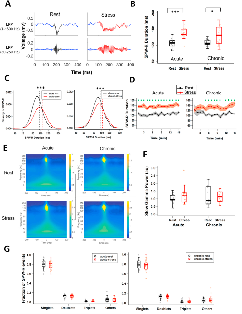
Fig. 2.
CA1 SPW-R duration differs between rest and stress states. (A) Representative examples of local field potential (LFP) for non-filtered (top) and filtered (bottom) SPW-R events recorded during rest-state (left) and stress-state (right) from CA1 stratum pyramidale. (B) SPW-R duration differs between rest-state and stress-state; (two-way ANOVA: behaviour-state, F(1, 61) = 34.035, p = 2.22 × 10⁻⁷; day, F(1, 61) = 0.419, p = 0.520; behaviour-state x day, F(1, 61) = 1.813, p = 0.183; Tukey's HSD: acute-rest vs acute-stress, p = 2.07 × 10⁻⁵, chronic-rest vs chronic-stress, p = 0.0137). (C) Distributions of the duration of SPW-Rs differs between behaviour states on first day (left: acute-rest vs acute-stress, Kolmogorov-Smirnov test, D = 0.236, p < 2.22 × 10⁻¹⁶) and last day (right: chronic-rest vs chronic-stress, Kolmogorov-Smirnov test, D = 0.113, p < 2.22 × 10⁻¹⁶) showed a rightward shift. Dotted vertical lines represent median values. (D) Temporal dynamics of averaged SPW-R duration (1-min bins) differ between behaviour states on the first day (left: LMMs; behaviour-state, F(1, 447) = 290. 40, p < 2.22 × 10⁻¹⁶; time, F(14, 447) = 0.757, p = 0.716; behaviour-state x time, F(14, 447) = 0.447, p = 0.958). Similarly, on the last day, SPW-R duration increased during stress (right: LMMs; behaviour-state, F(1, 412) = 94.08, p < 2.22 × 10⁻¹⁶; time: F(14, 412) = 1.19, p = 0.276; behaviour-state x time, F(14, 412) = 0.631, p = 0.839). (E) Averaged peri-SPW-R wavelet spectrograms during acute-rest (top left), acute-stress (bottom left), chronic-rest (top right) and chronic-stress (bottom right). (F) Low gamma (17–40Hz) power during SPW-R events does not differ between behaviour-states (two-way ANOVA: behaviour-state, F(1, 61) = 0.80, p = 0.38; day, F(1, 61) = 0.008, p = 0.928; behaviour-state x day, F(1, 61) = 0.105, p = 0.75). (G) Fraction of different types of ripple bursts during acute stress (two-way ANOVA: behaviour-state, F(1, 124) = 0.374, p = 0.542; category, F(3, 124) = 156.68, p < 2.22 × 10⁻¹⁶; behaviour-state x category, F(3, 124) = 0.211, p = 0.89; Tukey's HSD: acute-rest vs acute-stress: singlets, p = 0.999; doublets, p = 0.998; triplets, p = 0.999; others, p = 0.996) and chronic stress (two-way ANOVA: behaviour-state, F(1, 120) = 0.068, p = 0.795; category, F(3, 120) = 147.2, p < 2.22 × 10⁻¹⁶; behaviour-state x category, F(3, 124) = 0.371, p = 0.774; Tukey's HSD: chronic-rest vs chronic-stress: singlets, p = 1.0; doublets, p = 0.999; triplets, p = 0.967; others, p = 1.0). All box plots represent median and 25th-75th percentiles, with whiskers extending to the extreme data points. Circles depict rest-state (black) stress-state (red). *p < 0.05, **p < 0.01, ***p < 0.001. Acute-rest: n = 7220 SPW-Rs, N = 17 mice; acute-stress: n = 9851 SPW-Rs, N = 16 mice; chronic-rest: n = 7041 SPW-Rs, N = 16 mice; chronic stress: n = 8978 SPW-Rs, N = 16 mice). (For interpretation of the references to colour in this figure legend, the reader is referred to the Web version of this article.)

