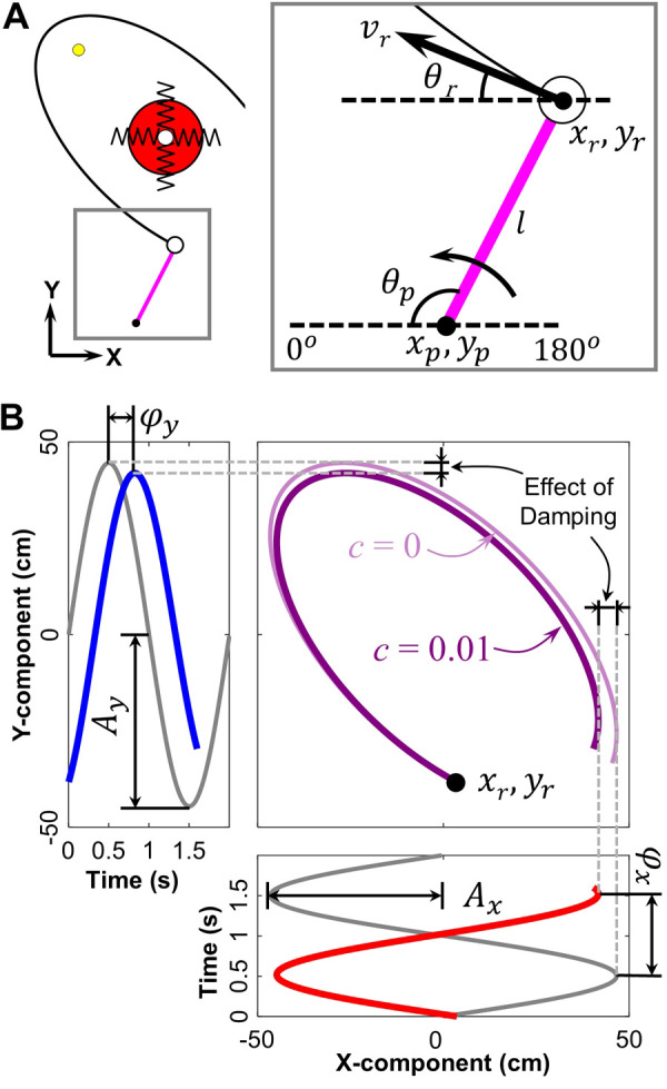
Figure 2.

Calculation of the ball trajectory. A: top-down view on the workspace, the springs visualize that the ball trajectory was modeled by two orthogonal springs. Execution variables of the ball trajectory in the two-dimensional (2D) workspace: x_p, y_p is the 2D position of the lever arm’s pivot; θ_p is the angle of the lever arm; l is the length of the lever arm; x_r and y_r is the 2D position of the ball release; v_r and θ_r are execution variables used to calculate the ball trajectory. The thick arrow indicates the direction of the arm movement for the throw. B: simulation of the ball trajectory. Gray curves denote y = A_x sin(x) and y = A_y sin(x). Red and blue curves are the x- and y-component of the ball trajectory with a phase shift and added damping, producing the trajectories in the x-y workspace. The dark purple trajectory is the resulting ball trajectory, whereas the light purple trajectory shows the trajectory without damping for reference.