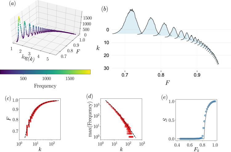
Fig. 5. Feature-enriched percolation of the SIS model.

We integrate the dynamical Eq. (19) for a reshuffled Barabási–Albert⁷⁰, with m = 3 and system size N = 2000. A non-normalized histogram of the pairs (k_i, F_i), where the feature value is F_i = x_i(t → ∞), is shown in (a). The input data for the histogram comes from 100 independent realizations. In (b), ridge plot of the 25 first curves of the histogram, i.e., those with the lowest degree and highest peaks. The bell shape behavior with varying mean, standard deviation, and peak height can clearly be appreciated. In (c), projection of the k − F plain, together with the expressions μ_F(k) (see text) given by the Bayesian machine scientist method. The standard deviation σ_F(k) is not shown because it visually overlaps μ_F(k) for large k. The expressions are ${\mu }_F\left(k\right)=\exp \left(a_1/\left(b_1-k\right)\right)$ and ${\sigma }_F\left(k\right)=\exp \left(a_2/\left(b_2-k\right)\right)-{\mu }_F\left(k\right)$, and have been obtained imposing only one free parameter per function, namely v = − 1.1641 and w = 0.4317. The constants in the exponential are given by a₁ = − v, $b_1=-{\cosh }^v\left(v^2\right)$, a₂ = 2w and $b_2=-{\cos }^2\left(w\right)$. d To find the height of the probability peaks we use the BMS on the pairs of variables $\left(k,\max \left(P\left(F\mid k\right)\right)\right)$, indicated by points, obtaining $h\left(k\right)=a_3{\left(x\left(b_3+x\right)\right)}^{-1}$ where the free parameter is t = 26.1442 and the constants in the function are $a_3={\tan }^t\left(t\right)/2$ and b₃ = t/2, indicated by the solid line. In (e), feature-enriched percolation of the SIS model, with the simulation (points) and the theoretical curve obtained from Eq. (21). Each point in (d) is averaged over 100 independent realizations of the dynamics.