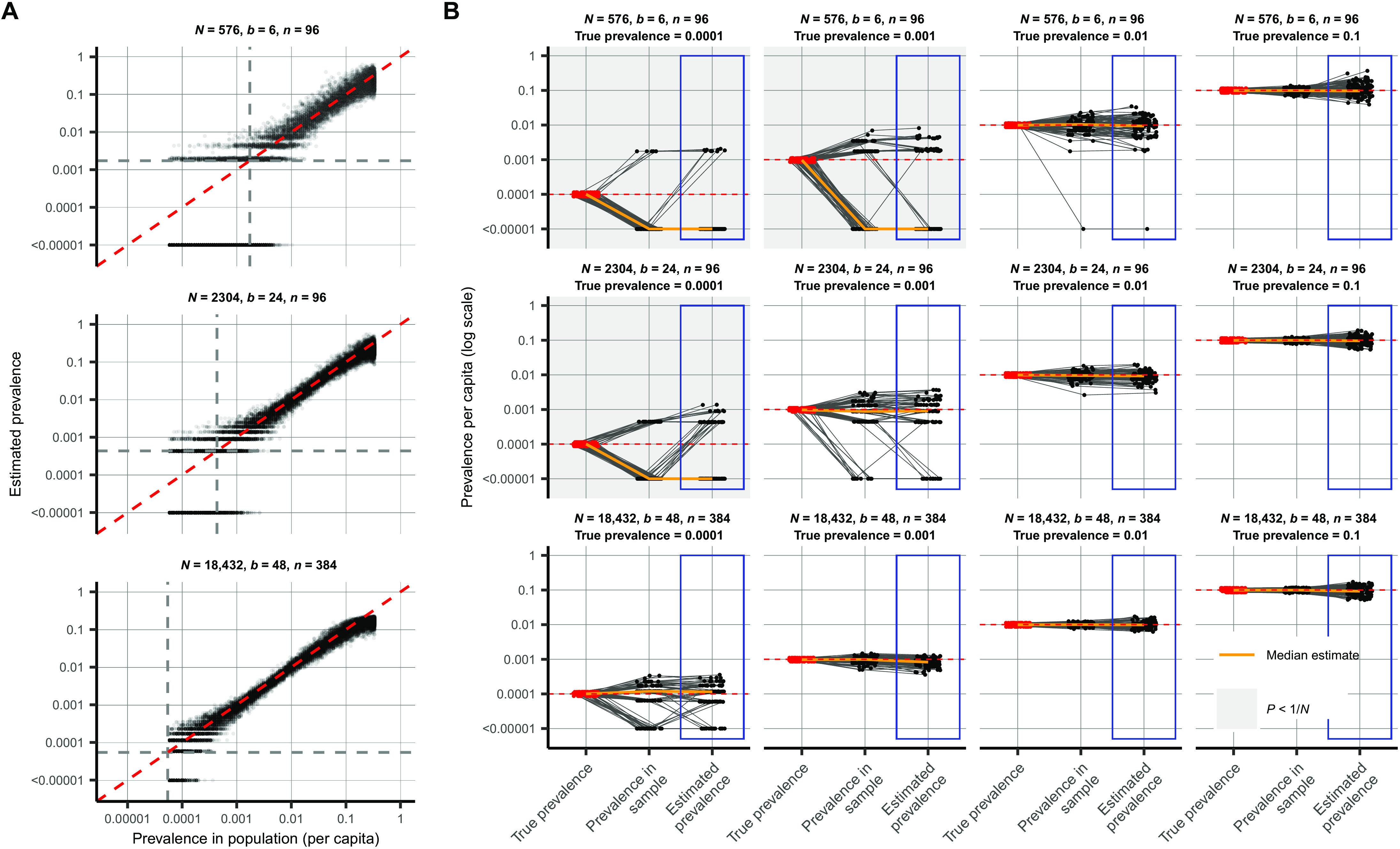
Fig. 3. Estimating prevalence from a small number of pooled tests.

In prevalence estimation, a total of N individuals are sampled and partitioned into b pools (with n = N/b samples per pool). The true prevalence in the entire population varies over time with epidemic spread. Population prevalences shown here are during the epidemic growth phase. (A) Estimated prevalence (y axis) and true population prevalence (x axis) using 100 independent trials sampling N individuals at each day of the epidemic. Each facet shows a different pooling design (additional pooling designs shown in fig. S1). Dashed gray lines, one divided by the sample size, N. (B) For a given true prevalence (top label, red points and horizontal dashed red line), estimation error is introduced both through binomial sampling of positive samples (prevalence in sample) and inference on the sampled viral loads (estimated prevalence, blue boxes). Each set of three connected dots shows one simulation, with points slightly jittered on the x axis for visibility. Horizontal lines indicate accurate inference. The orange line shows the median across 100 simulations. Each panel shows the results from a single pooling design at the specified true prevalence. Sampling variation is a bigger contributor to error at low prevalence and low sample sizes. When prevalence is less than one divided by N (gray-shaded panels), inference is less accurate due to the high probability of sampling only negative individuals or inclusion of false positives.