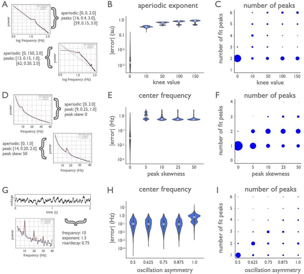
Extended Data Figure 3 |. Algorithm performance on simulated data that violate model assumptions.

(A-C) Power spectra were simulated across a broader frequency range (1–100 Hz), with two peaks, one in a low range, and one in a high range (see Methods), across five distinct knees values (1000 spectra per knee value), with a fixed noise level (0.01). Power spectra were parameterized in the ‘fixed’ aperiodic mode (without a knee) to evaluate how sensitive performance is to aperiodic mode. (A) Example power spectra with simulation parameters as aperiodic [offset, knee, exponent] and periodic [center frequency, power, bandwidth], showing spectra with knee values of 0 and 150, both fit in the ‘fixed’ aperiodic mode. (B) Absolute error of algorithmically identified aperiodic exponent, across spectra with different knee values. Notably, exponent reconstruction is high when spectra with knees are fit without a knee parameter. (C) The number of peaks fit by the model, across knee values. Note that all spectra in this group have two peaks, indicating here that the presence of knee’s in ‘fixed’ mode leads to overfitting peaks. (D-F) A distinct set of simulations were created in which power spectra were created with asymmetric or skewed peaks (see Methods), across five distinct skew levels (1000 spectra per skew level). (D) Example simulated spectra, showing two different skew levels. (E) Absolute error of algorithmically identified peak center frequency, across peak skewness values. (F) The number of peaks fit by the model, across peak skewness. Note that all spectra in this set have one peak. (G-I) A distinct set of simulations, in which time series were generated with asymmetric oscillations in the time domain, from which power spectra were calculated (see Methods), across five distinct levels of oscillation asymmetry (1000 spectra per asymmetry value). (G) Example simulation of an asymmetric oscillation, simulated in the time domain, and the associated power spectrum. Note that the power spectrum displays harmonic peaks. (H) Absolute error of algorithmically identified peak center frequency, across oscillation asymmetry values. (I) The number of peaks fit by the model, compared across oscillation asymmetry values. Note that these simulations all contained one oscillation in the time domain. All violin plots show full distributions, where small white dots represent median values and small box plots show median, first and third quartiles, and ranges. Note that the error axis is log-scaled in B,E,H.