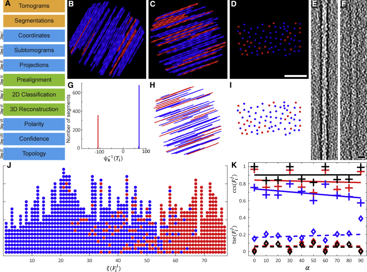
Figure 1.

Polarity determination of modeled actin bundles

(A) The workflow of APT consists of consecutive modules. The orange modules symbolize the required input data. The blue modules were implemented in MATLAB, and the green modules were executed in RELION.

(B) Top view of one of the modeled actin bundles, which were used for the validation of APT. The bundles were rendered without noise for visualization purposes. Here the angle $\alpha$ between bundle and tilt axis is 30°, and the fraction ${\rho }_r$ of actin filaments that are oriented in the opposite direction (red colored filaments) was set to 0.1.

(C) Top view of an additional bundle with $\alpha$ increased to 70°, and ${\rho }_r$ to 0.3.

(D) The same bundle seen from the side with the viewing axis adjusted parallel to the filaments. The distance between the filaments is 10–37 nm. Scale bar, 100 nm.

(E and F) (E) In order to quantify the impact of noise on the precision of APT, the bundles were modeled with defined SNRs. The depicted bandpass filtered slice of a filament was extracted from a bundle with SNR = ${10}^{-3}$. For comparison, the filament shown in (F) originates from a bundle with SNR = ${10}^{-4}$. Scale bar, 10 nm.

(G) The modeled bundles were processed with APT. The plot shows the resulting ${\text{ψ}}_k^{-1}\left(T_i\right)$ histogram of the bundle displayed in (C). Segments in the blue peak mainly originate from blue filaments, and the opposite for the red peak. The filaments point with their plus ends in opposite directions, so the peaks are separated by 180°. Since ${\rho }_r$ was set to 0.3 in this bundle, the number of segments in the red peak is $\approx$30% of the total number of segments.

(H and I) (H) The line plot shows the filament positions and polarities of the bundle, shown in (C), as recovered by APT. It was affected with SNR = ${10}^{-3}$; however, in this case the match between original and recovered bundle (the side view is shown in [I], and can be compared with [D]) is almost error free.

(J) Here the $\xi \left(F_i^j\right)$ vectors of the recovered bundle are depicted. Segments that originate from the same filament are plotted as columns of circles. The color scheme reflects to which peak the segments were assigned in the ${\text{ψ}}_k^{-1}\left(T_i\right)$ histogram, shown in (G), and the $\xi \left(F_i^j\right)$ vectors are sorted according to their fraction of segments linked to the blue peak. In this representation of the filaments, segments with incorrect orientation determination appear as distortions of otherwise uniformly colored columns.

(K) Three modeled datasets with three different SNRs were produced, each comprising 10 bundles with varying orientation $\alpha$ between $0°$ and $90°$. The data were processed with APT and the $ccs\left(F_i^j\right)$ and $tse\left(F_i^j\right)$ values were analyzed. Each cross in the plot marks the average of all $ccs\left(F_i^j\right)$ values in a bundle and diamond symbols indicate averaged $tse\left(F_i^j\right)$ values per bundle. The SNR of the respective dataset can be identified by the color scheme: black, SNR = ${10}^{-2}$; red, SNR = ${10}^{-3}$; and blue, SNR = ${10}^{-4}$, respectively. Linear regression lines are depicted as solid or dashed lines.

See also Figures S1 and S2.