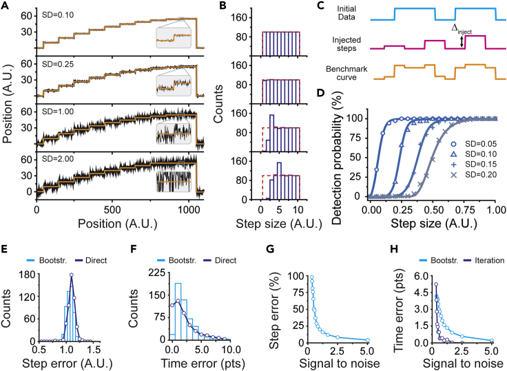
Figure 5.
Testing the detection limits of AutoStepfinder
(A) Simulated time trajectories that were exposed to various noise levels to benchmark the AutoStepfinder algorithm. The data start with a step of 10 arbitrary units (a.u.), the subsequent steps decrease by 1 a.u. until the smallest step size of 1 a.u. is reached. This idealized trajectory was repeated 100 times, resulting in a dataset in which each step size occurred 100 times.
(B) Distribution of step sizes of the simulated trajectories, obtained through the AutoStepfinder algorithm. The red dashed lines indicate the position of each bin when 100% of the steps are correctly identified.
C) Schematic of the step injection test. To quantify the probability that AutoStepfinder would detect steps with a certain size (Δinject), steps were injected (pink curve, middle) into an existing trajectory (blue curve, top) to generate a benchmark curve (orange curve, bottom).
(D) Histogram of the detection probability of step sizes at various noise levels (SD). Solid lines represent sigmoidal fits to the data.
(E) Histogram showing the distribution of the 95% confidence intervals of the step sizes (cyan bars) obtained by bootstrap analysis. The line (purple) indicates the deviation of the fit from the ground truth.
(F) Histogram showing the distribution of the 95% confidence intervals of the plateaus lengths (cyan bars) obtained by bootstrap analysis. The line (purple) indicates the deviation of the fit from the ground truth.
(G) Relation between the SNR and the error in the determined steps.
(H) Relation between the SNR and the error in the determined plateaus (cyan line). The purple line indicates the deviation between the final fit and a local refit at various noise levels (iteration error).
Also see Figure S4.

