. 2021 May 20;10:e63711. doi: 10.7554/eLife.63711

Figure 3. Performance in the basic task was indistinguishable across laboratories.

(a) Psychometric curves across mice and laboratories for the three sessions at which mice achieved proficiency on the basic task. Each curve represents a mouse (gray). Black curve represents the example mouse in Figure 1. Thick colored lines show the lab average. (b) Average psychometric curve for each laboratory. Circles show the mean and error bars ± 68% CI. (c) performance on easy trials (50% and 100% contrasts) for each mouse, plotted per lab and over all labs. Colored dots show individual mice and boxplots show the median and quartiles of the distribution. (d-e) Same, for contrast threshold and bias. (f) Performance of a Naive Bayes classifier trained to predict from which lab mice belonged, based on the measures in (c-e). We included the timezone of the laboratory as a positive control and generated a null-distribution by shuffling the lab labels. Dashed line represents chance-level classification performance. Violin plots: distribution of the 2000 random sub-samples of eight mice per laboratory. White dots: median. Thick lines: interquartile range.

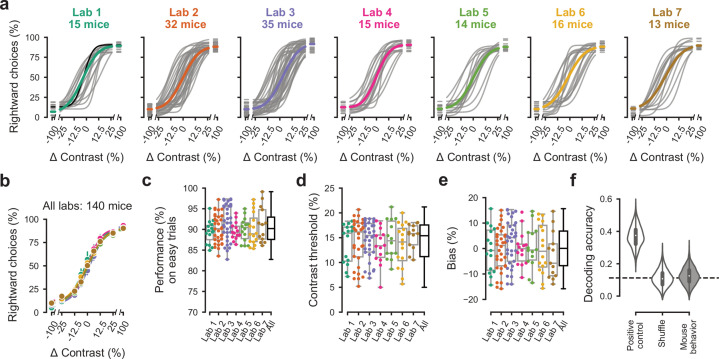
Figure 3.

Figure 3—figure supplement 1. Mouse choices were no more consistent within labs than across labs.

Figure 3—figure supplement 1.

To measure the similarity in choices across mice within a lab, we computed within-lab choice consistency. For each lab and each stimulus, we computed the variance across mice in the fraction of rightward choices. We then computed the inverse (consistency) and averaged the result across stimuli. (a) Within-lab choice consistency for the basic task (same data as in Figure 3) for each lab (dots) and averaged across labs (line). This averaged consistency was not significantly higher (p=0.73) than a null distribution generated by randomly shuffling lab assignments between mice and computing the average within-lab choice variability 10,000 times (violin plot). Therefore, choices were no more consistent within labs than across labs. (b) Same analysis, for the full task (same data as in Figure 4). Within-lab choice consistency on the full task was not higher than expected by chance, p=0.25. In this analysis we computed consistency separately for each stimulus and prior block before averaging across them. Choice consistency was higher on the full task than the basic task; this likely reflects both increased training on the task, and a stronger constraint on choice behavior through the full task’s block structure. (c) As in a, b, but measuring the within-lab consistency of ‘bias shift’ between the 20:80 and 80:20 blocks (as in Figure 4d,e). Within-lab consistency in bias shift was not higher than expected by chance (p=0.31).
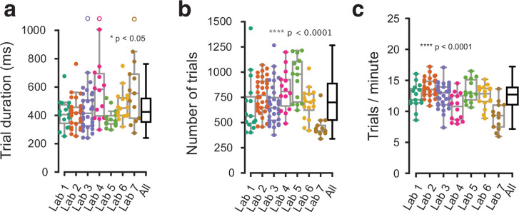
Figure 3—figure supplement 2. Behavioral metrics that were not explicitly harmonized showed small variation across labs.

Figure 3—figure supplement 2.

(a) Average trial duration from stimulus onset to feedback, in the three sessions at which a mouse achieved proficiency in the basic task, shown for individual mice (dots) and as a distribution (box plots). (b) Same, for the average number of trials in each of the three sessions. (c) Same, for the number of trials per minute. Each dot represents a mouse, empty dots denote outliers outside the plotted y-axis range.
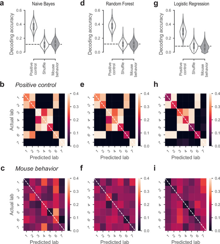
Figure 3—figure supplement 3. Classifiers could not predict lab membership from behavior.

Figure 3—figure supplement 3.

(a) Classification performance of the Naive Bayes classifier that predicted lab membership based on behavioral metrics from Figure 3. In the positive control, the classifier had access to the time zone in which a mouse was trained. In the shuffle condition, the lab labels were randomly shuffled. (b) Confusion matrix for the positive control, showing the proportion of occurrences that a mouse from a given lab (y-axis) was classified to be in the predicted lab (x-axis). Labs in the same time zone from clear clusters, and Lab seven was always correctly predicted because it’s the only lab in its time zone. (c) Confusion matrix for the classifiers based on mouse behavior. The classifier was generally at chance and there was no particular structure to its mistakes. (d-f) Same, for the Random Forest classifier. (g–i) Same, for the Logistic Regression classifier.
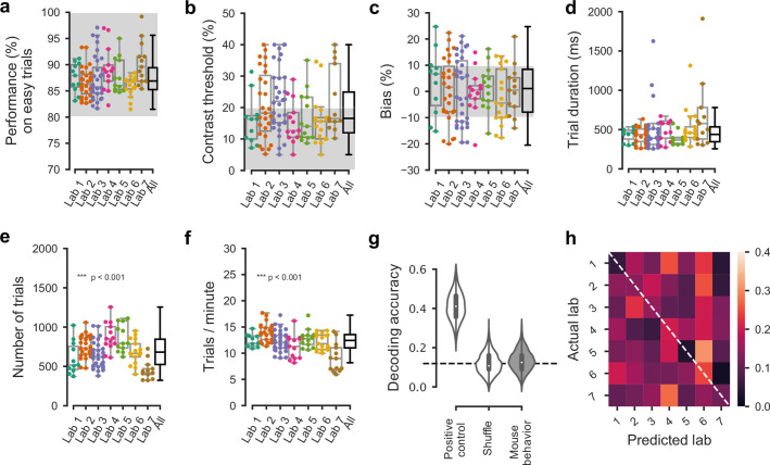
Figure 3—figure supplement 4. Comparable performance across institutions when using a reduced inclusion criterion (>=80% performance on easy trials).

Figure 3—figure supplement 4.

(a) Performance on easy trials (50% and 100% contrasts) for each mouse, plotted over all labs (n = 150 mice). Colored dots show individual mice and boxplots show the median and quartiles of the distribution. (b–f) Same, for (b) contrast threshold, (c) bias, (d) trial duration and (e–f) trials completed per session. As it was the case with our standard inclusion criteria (Figure 3—figure supplement 2), there was a small but significant difference in the number of trials per session across laboratories. All other measured parameters were similar. (g) Performance of a Naive Bayes classifier trained to predict from which lab mice belonged, based on the measures in a-c. We included the timezone of the laboratory as a positive control and generated a null-distribution by shuffling the lab labels. Dashed line represents chance-level classification performance. Violin plots: distribution of the 2000 random sub-samples of 8 mice per laboratory. White dots: median. Thick lines: interquartile range. (h) Confusion matrix for the classifiers based on mouse behavior with reduced inclusion criteria. The classifier was at chance and there was no particular structure to its mistakes.
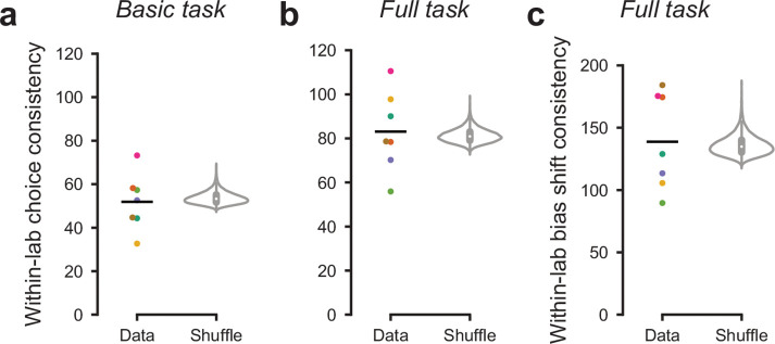
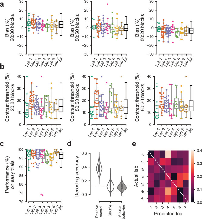
Figure 3—figure supplement 5. Behavior was indistinguishable across labs in the first 3 sessions of the full task.

Figure 3—figure supplement 5.

For the first 3 sessions of performing the full task (triggered by achieving proficiency in the basic task, defined by a set of criteria, Figure 1—figure supplement 1d). (a) Bias for each block prior did not vary significantly over labs (Kruskal-Wallis test, 20:80 blocks; p=0.96, 50:50 block; p=0.96, 80:20 block; p=0.89). (b) The contrast thresholds also did not vary systematically over labs (Kruskal-Wallis test, 20:80 block; p=0.078, 50:50 block; p=0.12, 80:20 block; p=0.17). (c) Performance on 100% contrast trials neither (Kruskal-Wallis test, p=0.15). (d) The Naive Bayes classifier trained on the data in (a–c) did not perform above chance level when trying to predict the lab membership of mice. (e), Normalized confusion matrix for the classifier in (d).