Towards theoretical spectroscopy with error bars: systematic quantification of the structural sensitivity of calculated spectra

Abstract

Molecular spectra calculated with quantum-chemical methods are subject to a number of uncertainties (e.g., errors introduced by the computational methodology) that hamper the direct comparison of experiment and computation. Judging these uncertainties is crucial for drawing reliable conclusions from the interplay of experimental and theoretical spectroscopy, but largely relies on subjective judgment. Here, we explore the application of methods from uncertainty quantification to theoretical spectroscopy, with the ultimate goal of providing systematic error bars for calculated spectra. As a first target, we consider distortions of the underlying molecular structure as one important source of uncertainty. We show that by performing a principal component analysis, the most influential collective distortions can be identified, which allows for the construction of surrogate models that are amenable to a statistical analysis of the propagation of uncertainties in the molecular structure to uncertainties in the calculated spectrum. This is applied to the calculation of X-ray emission spectra of iron carbonyl complexes, of the electronic excitation spectrum of a coumarin dye, and of the infrared spectrum of alanine. We show that with our approach it becomes possible to obtain error bars for calculated spectra that account for uncertainties in the molecular structure. This is an important first step towards systematically quantifying other relevant sources of uncertainty in theoretical spectroscopy.

Uncertainty quantification is applied in theoretical spectroscopy to obtain error bars accounting for the structural sensitivity of calculated spectra.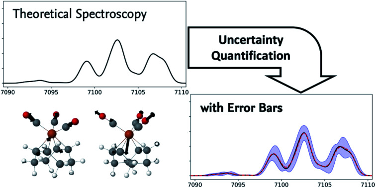

1. Introduction

The quantum-chemical calculation of molecular spectra has nowadays become an essential tool for determining the structure of molecules.¹ In many cases, structural information can only be extracted from experimental spectra by combining them with computations.² Examples include the elucidation of the gas-phase structure of polypeptides with vibrational spectroscopy,^3–7 the assignment of the absolute configuration of chiral molecules with chiroptical spectroscopic techniques,^8–11 and the identification of active species and catalytic intermediates with X-ray spectroscopy.^12–15

While in some cases, high-resolution spectroscopic experiments can resolve the individual spectroscopic transition, this is usually not the case for most common applications that aim at obtaining structural information from spectroscopic experiments, such as those mentioned above. Instead, the quantity of interest is the spectral intensity as a function of the radiation energy, σ(E), in a relevant energy range, which is usually calculated as,

1

where E_n and f_n are the excitation energy and oscillator strength of the n-th excitation, respectively, which are provided by quantum-chemical calculations, and G(E) is a suitable—usually empirical—line broadening function. To extract structural information from experimental spectra (e.g., in the examples cited above), the spectral intensity σ(E) calculated for suitable structural models is compared to a measured spectrum, and conclusions are drawn based on the agreement or disagreement of experiment and theory.

However, quantum-chemical calculations are affected by numerous uncertainties and in general the agreement between experiment and computation cannot be expected to be perfect. Sources of uncertainties include the structure of the molecular model, the description of environment effects, and errors of the quantum-chemical methods used for calculating spectra. The comparison of measured and calculated spectra thus requires carefully judging these uncertainties. To this end, one generally relies on the often rather subjective judgement of computational chemists.

Methods for the systematic assessment of uncertainties in computer simulations are developed in the field of uncertainty quantification, which is a subfield of applied mathematics that has developed in the past decades (for textbooks, see, e.g., ref. 16 and 17). It provides tools that are widely used in simulation science.^18,19 However, their application in quantum chemistry is only just emerging (for a recent review, see ref. 20). For quantifying uncertainties in reaction energies that are due to errors of approximate density-functional theory (DFT), Nørskov, Sethna, Jacobsen, and coworkers have developed the Bayesian error estimation exchange–correlation functional (BEEF),^21–24 while Reiher and coworkers extended this approach by parametrizing problem-specific exchange–correlation functionals with built-in error estimation.^25,26 Recently, the BEEF family of xc functionals has been applied to quantify uncertainties in calculated vibrational frequencies.²⁷ Several groups have addressed the assignment of uncertainties to the parameters of calibration models,²⁸ such as scaling factors for harmonic vibrational frequencies,^29,30 or linear regression models for the quantum-chemical calculation of Mössbauer isomer shifts.³¹ Similarly, uncertainties in the parameters of the semi-empirical PM7 method,³² of Grimme's D3 dispersion correction,³³ and of neural networks for the exploration of chemical space³⁴ have been assessed.

Here, our objective is to further explore the application of methods of uncertainty quantification to the quantum-chemical calculation of molecular spectra. Within a chosen quantum-chemical model, the calculated spectral intensity will depend on the input molecular structure R that is used in the quantum-chemical calculation, i.e.,Here, we specifically chose σ(E) instead of the positions and/or intensities of individual peaks as quantity of interest, because in many spectroscopic experiments for complex chemical systems the individual transitions are not resolved.

Previously, some authors have addressed the quantification of uncertainties introduced by approximations in the quantum-chemical model on spectroscopic properties.^27,29–31 Here, we aim at systematically quantifying a further source of uncertainty, namely the dependence of σ(E; R) on the input molecular structure.³⁵ The structural sensitivity presents a challenging case because the calculated spectrum depends on a rather large number of independent parameters (i.e., the nuclear coordinates R). In this respect, it fundamentally differs from, e.g., uncertainties due to approximation in the quantum-chemical model, which are usually related to only a few parameters. Thus, while the structural sensitivity is only one of many relevant sources of uncertainty, it serves as a first step towards establishing a methodological framework that can be extended to other sources of uncertainty.

Specifically, we set out to establish “error bars” that account for the structural sensitivity of a calculated spectrum. In this paper, we present a methodology that allows us to answer the following two questions: (1) Given distortions ΔR of a reference structure R₀ with |ΔR| ≤ d_max, what is the range of calculated spectra σ(E; R₀ + ΔR)? (2) Given a probability distribution for distortions of a reference structure R₀, how can we characterize the resulting probability distribution for the calculated spectra? This can then be employed to obtain error bars for the calculated spectrum of the reference structure that either represent bounds on the calculated spectra of distorted structures or that quantify the uncertainty due to structural distortions in a statistical fashion.

We aim at developing a methodology that is generally applicable for any type of computational spectroscopy providing a spectral intensity σ(E) that can be compared to an experimental spectrum. To this end, we will consider typical applications in which structural information in extracted from the comparison of experimental and calculated spectra, such as X-ray emission spectroscopy (XES) of transition metal complexes, vibrational spectroscopy, and UV/Vis spectroscopy.

This work is organized as follows. In Section 2, we show how the structural distortions that are most influential for the calculated spectrum can be identified. This is then used in Section 3 to construct nonlinear surrogate models of the dependence of the calculated spectrum on the input molecular structure, and we use this model for analyzing the propagation of uncertainties in the molecular structure to the calculated spectrum in Section 4. In Sections 2–4, we illustrate our methodology for the calculated XES spectrum of iron pentacarbonyl Fe(CO)₅ as a test case. Results for further test cases covering XES, UV/Vis spectroscopy, and infrared spectroscopy are presented in Section 5. Finally, in Section 6 we present our conclusions as well as perspectives for future work. The computational details are given in the Appendix.

2. Identification of influential structural distortions

As the space of possible molecular structures R for a given atomic composition is intractably vast and because large parts of this space are chemically irrelevant, we only aim at analyzing the structural sensitivity of calculated molecular spectra around a chosen reference structure R₀, i.e., R = R₀ + ΔR. Usually, this will be the structure obtained as a minimum on the potential energy surface, but other choices are also possible. In the following, we will consider distortions of this reference structure,

2

where e_Iα is a unit vector for a displacement of the I-th nucleus in α = (x, y, z) direction, i.e., our target is the change in the spectral intensity

3

The dependence of the calculated spectrum on the molecular structure around R can the be subjected to a local sensitivity analysis,³⁶ which considers the linearized model

4

with the linear structural sensitivity with respect to a Cartesian displacement in e_Iα-direction,

5

This linear structural sensitivity can be calculated by numerical differentiation, i.e., by calculating the spectrum for displaced molecular structures.³⁵ Here, we employ a symmetric two-point formula [see eqn (5)] and a displacement of h = 0.5 pm. Tests included in our earlier work showed that this numerical derivative is rather insensitive with respect to the magnitude of the displacement and found that h = 0.5 pm should be a reasonable choice.³⁵ Overall, the calculation of the linear structural sensitivity for all 3N Cartesian displacements requires 6N calculations of spectra for displaced structures.

To identify the linear combinations of structural distortions that are most influential on the calculated spectrum, a principal component analysis³⁷ can be performed. After discretizing the energy axis of the calculated spectrum E = {E_j} (with j = 1, …, M, where M ≫ 3N), the linear structural sensitivities can be collected in a (3N × M)-matrix X with

X_Iα,j = δσ_Iα(E_j), 6

i.e., the rows of this matrix contain the discretized linear structural sensitivities with respect to the 3N Cartesian displacements. Here, we use M = 10 000 evenly spaced points in the relevant energy range. With the singular value decomposition of X = U·S·V^T, we obtain

U^T·X = S·V^T, 7

where U is an orthogonal (3N × 3N)-matrix, V is an orthogonal (M × M)-matrix, and the (3N × M) diagonal matrix S contains the 3N singular values s_k on its diagonal.

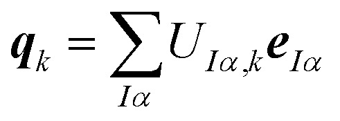
Here, the columns of U define principal component distortions,

8

i.e., q_k is the unit vectors of a collective distortion corresponding to the k-th principal component. These principal component distortions {q_k} constitute an alternative basis of the full space of structural distortions, in which the displacement vector ΔR can be expressed as,

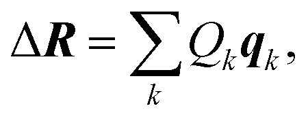9

where Q_k is the displacement in direction of the collective coordinate q. The vector Δq = (Q₁, Q₂, …)^T = UΔR describes the displacement in the basis of our new collective coordinates. Note that despite the notational and conceptual similarity, the collective coordinates {q_k} describing the principal component distortions and the displacements Q_k differ from the normal coordinates and normal modes appearing in theoretical vibrational spectroscopy (see Section S1 in the ESI† for a detailed analysis). Nevertheless, because of this analogy we will refer to the collective coordinates {q_k} as sensitivity modes in the following.

The linear structural sensitivities can now also be expressed with respect to the principal component distortions as

10

By comparing with eqn (7), we find

11

i.e., the k-th column of the matrix V multiplied by the k-th singular value s_k corresponds to the discretized principal component structural sensitivity δσ^PC_k with respect to distortions along the sensitivity mode q_k. Note that because V is an orthogonal matrix, its columns are normalized. Therefore,

12

and the norm of δσ^PC_k is proportional to the corresponding singular value s_k. Thus, the k-th singular value provides a quantitative measure for the linearized influence of distortions along sensitivity mode q_k on the calculated spectrum.

Altogether, the linearized model of eqn (4) can now be expressed as

13

which makes it possible to truncate the sum over principal components by neglecting the contributions that correspond to small singular values. In general, the linearized dependence of the calculated spectra on structural distortions can thus be described accurately by including only a few displacements along the k_max most influential sensitivity modes q₁, …, q_kmax. Note that the resulting linearized model will depend on the choice of the quantity of interest, i.e., on the relevant energy range and on the parameters used for an empirical line broadening.

As an example, we consider the structural sensitivity of the calculated XES spectrum of Fe(CO)₅. XES is widely used to obtain insights into the geometrical and electronic structure at transition metal centers from the combination of experimental and theoretical spectroscopy.^12–15 Fe(CO)₅ is a prototypical transition metal complex, and its XES spectrum has been previously studied both experimentally and computationally. As the calculation of XES spectra within a ΔDFT approximation³⁸ only requires a ground-state calculation, it constitutes an ideal first test case. For this example, we already explored the dependence on manually selected structural distortions in our previous work.³⁵ An in-depth experimental and computational study of the XES spectrum of Fe(CO)₅ can be found in ref. 39.

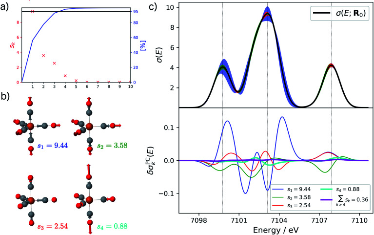
Starting from the minimum energy structure of Fe(CO)₅, we calculated the linear structural sensitivity δσ_Iα(E) with respect to all 33 Cartesian displacements by numerical differentiation and performed the principal component analysis outlined above. The resulting singular values are plotted in Fig. 1a. We find that the four largest singular values (s₁ = 9.44, s₂ = 3.58, s₃ = 2.54, s₄ = 0.88) account for over 95% of the sum of all singular values. The sum of the remaining 29 singular values amounts to only 0.36. The corresponding sensitivity modes q_k are visualized in Fig. 1b and the corresponding principal component structural sensitivities δσ^PC_k are shown in Fig. 1c.

Fig. 1. Principal component analysis of the linearized structural sensitivity of the calculated XES spectrum of Fe(CO)₅. (a) Singular values s_k (red) and sum of the singular values (blue) in descending order. (b) Visualization of the sensitivity modes q_k corresponding to the four largest singular values. (c) Calculated XES spectrum (upper panel) and principal component structural sensitivities δσ^PC_k (lower panel). The color-coded shaded areas indicate the linearized change in the calculated spectrum for distortions of Q_k = ±4 pm.

For the largest singular value s₁, the sensitivity mode q₁ is given by a collective symmetric C O stretching coordinate. Distorting the molecular structure along this mode will mainly affect the position and intensity of the first peak as well as the intensity of the second peak in the calculated XES spectrum, while it leaves the third peak mostly unchanged (see blue graphs in Fig. 1c). The second sensitivity mode q₂ corresponds to a symmetric Fe–C stretching coordinate. A distortion along this mode will affect all three peaks, but to a much smaller extent than for the first sensitivity mode (see green graphs in Fig. 1c). The third and forth sensitivity modes q₃ and q₄ are asymmetric Fe–C and C O stretching coordinates, respectively, in which the distortions of the axial and equatorial ligands form an out-of-phase combination. Again, it is obvious form Fig. 1c (see red and cyan graphs) that the effect of a distortion along q₃ and q₄ further decreases, and is already almost negligible for q₄.

Finally, the lower panel of Fig. 1c also includes the sum of the principal component structural sensitivities corresponding to all remaining singular values (magenta line), which turns out to be negligible. Thus, a principal component analysis allows for a significant reduction of the dimensionality of the linearized change in the calculated spectrum,

δσ(E;ΔR) = δσ(E;Δq) ≈ δσ(E;Q₁, …, Q_kmax). 14

For the example of Fe(CO)₅ only four collective displacements Q₁, …, Q₄ along sensitivity modes instead of the full 33 Cartesian displacements ΔR_Iα are required for accurately describing the dependence of the calculated XES spectrum on the underlying molecular structure. All remaining principal component distortions turn out to be non-influential within the linearized model.

3. Construction of nonlinear surrogate models

Based on a principal component analysis, the dimensionality of a linearized model can be significantly reduced by only considering the most influential principal component distortions and neglecting non-influential distortions. This can now be used as starting point for constructing nonlinear surrogate models of the structural sensitivity of calculated spectra within this reduced space, i.e.,

Δσ(E;ΔR) ≈ Δσ(E;Q₁, …, Q_kmax). 15

The use of such a reduced space is based on the assumption that the sensitivity modes that are non-influential in the linearized model also only have a small influence when considering the full structural sensitivity. Additional tests to verify this assumption are presented in the ESI (Section S2).†

A general ansatz for a nonlinear surrogate model within the reduced space of the displacements that are most influential in the linearized model is given by

16

with the one-mode contributions

Δσ⁽¹⁾_k(E;Q_k) = Δσ(E;0, …,Q_k, …, 0), 17

two-mode contributions

Δσ⁽²⁾_kl(E;Q_k, Q_l) = Δσ(E;0, …, Q_k, …, Q_l, …, 0) − Δσ⁽¹⁾_k(E;Q_k) − Δσ⁽¹⁾_l(E;Q_l), 18

and possibly further higher-order contributions. In the literature on uncertainty quantification, this ansatz is referred to as high-dimensional model representation (HDMR)⁴⁰ and is closely related to the Sobol expansion.⁴¹ The specific form considered here is known as Cut-HDMR.⁴² In theoretical chemistry, such an ansatz is well known from the N-mode expansion commonly used in anharmonic theoretical vibrational spectroscopy and quantum dynamics.^43–46 Note that this ansatz is exact within our reduced space if all contributions up to order k_max are included, but generally a truncation at a lower order is used as an approximation. Furthermore, the Cut-HDMR expansion of eqn (16) provides the possibility for introducing further approximations to the individual one-mode, two-mode, and possibly higher-order contributions.

In the linearized model of eqn (13), two-mode and higher-order contributions are neglected while the one-mode contributions are approximated as

Δσ⁽¹⁾_k(E;Q_k) ≈ δσ^PC_k(E)Q_k. 19

To improve upon this linear approximation for the one-mode contributions, one can employ a Taylor expansion, i.e.,

20

Similarly, instead of neglecting the two-mode contributions, these could be approximated via a Taylor expansion,

21

Here, the quadratic term is the lowest order entering the two-mode contributions. The required higher derivatives can be calculated by numerical differentiation. As before, for the one-mode contributions we use a displacement of h = 0.5 pm in combination with a three-point finite-difference formula for the second derivative, a four-point formula for the third derivative, and possibly a five-point formula for the fourth derivative along one mode.

As an alternative to a Taylor expansion, the one-mode, two-mode, higher-order contributions could also be approximated by a discretized representation on a suitable grid of distortions in the relevant range. Note that the fact that the surrogate model is only constructed in the reduced space of the most influential sensitivity modes significantly reduces the number of additional quantum-chemical calculations of the spectrum for distorted structures that are required for its construction.

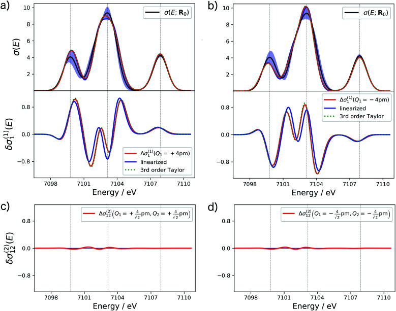
The accuracy of different approximations within a surrogate model can be assessed by comparing the change in the spectrum predicted by the model to the one obtained from a calculation of the spectrum for a distorted structure. For the example of the XES spectrum of Fe(CO)₅, such a comparison is shown for selected terms in Fig. 2.

Fig. 2. Analysis of the accuracy of different approximations of the one-mode and two-mode contributions to the structural sensitivity of the calculated XES spectrum of Fe(CO)₅. (a and b) One-mode contributions obtained from calculations for displaced structures with Q₁ = ±4 pm (solid red line) compared to a linearized approximation (solid blue line) and a 3rd order Taylor expansion (dashed green line). The top panels show the corresponding spectra while the lower panels show the change in the calculated spectra. (c and d) Two-mode contributions obtained from calculations for displaced structures with (i.e., |Δq| = 4 pm).

For the one-mode contributions, we consider a distortion of ±4 pm along the most influential sensitivity mode in Fig. 2a and b. The exact one-mode contribution obtained from a calculations of the spectrum for distorted structures (red line) is in good agreement with the linearized model (blue line), but some differences appear in the region of the first and second peak. When going to a 3rd order Taylor expansion (dashed green line), these differences disappear and an almost perfect agreement with the exact one-mode contribution is found on the scale of the figure. Fig. 2c and d shows the exact two-mode contribution obtained from calculating the spectrum for structures that were simultaneously distorted by |Δq| = 4 pm along the two most influential sensitivity modes. The plots show that these two-mode contributions are almost negligible.

Based on these tests, in the following we use a 3rd order Taylor expansion for the one-mode contributions and neglect all two-mode contributions. Of course, such a choice will have to be reassessed for different test cases. More systematic schemes for the construction of non-linear surrogate models that include additional terms on-the-fly as needed can also be envisioned.

4. Analysis of uncertainty propagation

A surrogate model of the change in the calculated spectrum Δσ(E;ΔR) can be evaluated for arbitrary structural distortions without significant computational effort. This now makes it possible to analyze the propagation of uncertainties in the molecular structure to uncertainties in the calculated spectrum.

First, we consider the molecular structures that can be obtained from the reference structure by distortions up to a given magnitude d_max, i.e., with |ΔR| ≤ d_max. As the transformation from Cartesian distortions to sensitivity modes is orthogonal, this is equivalent to |Δq| ≤ d_max. Such distortions will result in changes in the calculated spectrum, for which we want to determine upper and lower bounds. For a surrogate model expressed as HDMR expansion up to two-mode contributions we find,

22

with the analogous expression for the minimum. Note that on the right-hand side we applied the triangle inequality, i.e., the upper and lower bounds given by this equation are not tight.

The calculation of the maximum and minimum of the change in the spectrum is thus reduced to determining the maximum and minimum for the one-mode and two-mode contributions, i.e., for simple one- or two-dimensional functions. For the linearized model, only the one-mode contributions at the maximum displacements Q_k = ±d_max need to be considered. In the general case, the maximum and minimum can be found by sampling the one-mode and two-mode contributions in the relevant interval (e.g., using 100 evenly spaced points between −d_max and +d_max for the one-mode contributions).

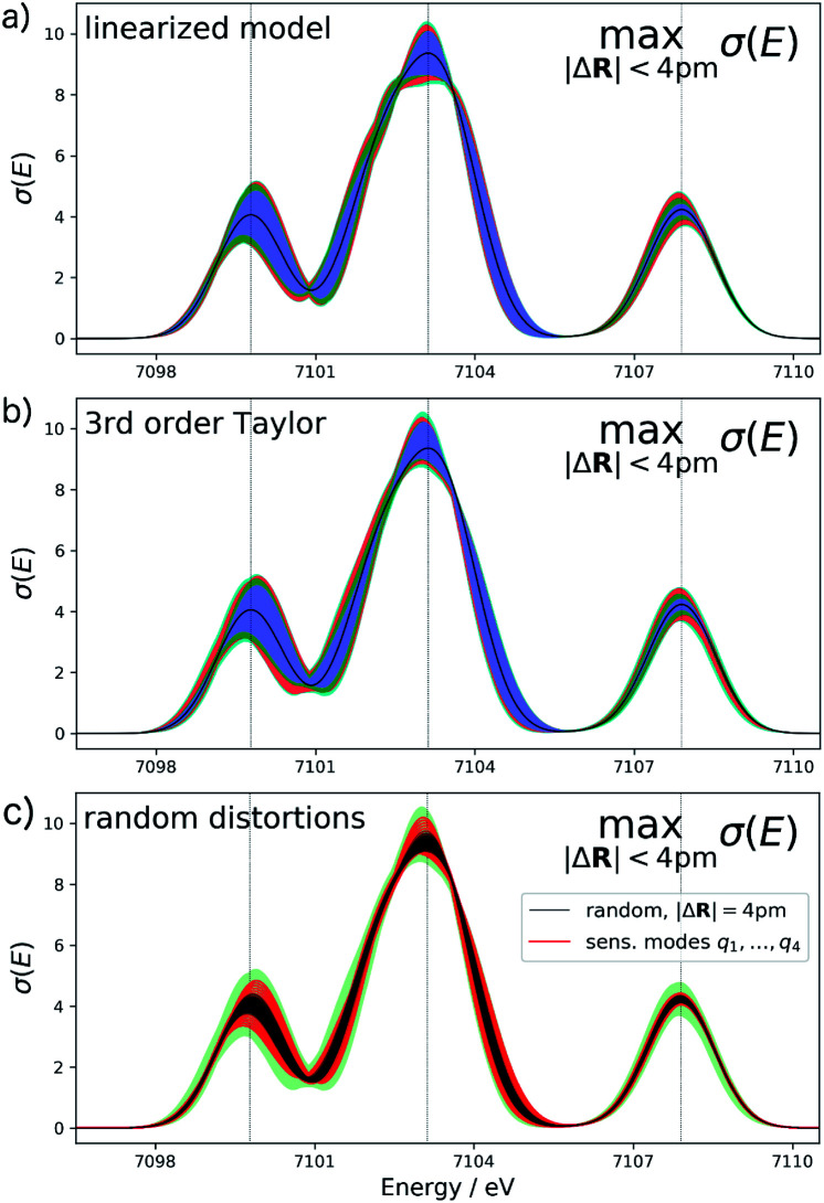
For the test case of the XES spectrum of Fe(CO)₅, the error bars for distortions of up to 4 pm calculated according to eqn (22) are shown in Fig. 3a for the linearized model and in Fig. 3b for a non-linear surrogate model based on a 3rd-order Taylor expansion for the one-mode contributions.

Fig. 3. Calculated XES spectrum of Fe(CO)₅ (black line) including error bars (shaded area) giving upper and lower bounds for distortions of the minimum energy reference structure with |ΔR| ≤ 4 pm. The different colors of the shaded area indicate the contributions of the four most influential sensitivity modes (q₁ blue; q₂ green, q₃ red, q₄ cyan). (a) Error bars calculated for the linearized surrogate model and (b) for the non-linear surrogate model based on a 3rd-order Taylor expansion for the one-mode contributions and neglecting two-mode and higher-order contributions. (c) Spectra calculated for 100 random distortions with |ΔR| = 4 pm (black lines) as well as 20 evenly spaced distortions between Q_i = ±4 pm along each of the four most influential sensitivity modes (red lines). The total error bars from (b) are included as green shaded area for comparison.

For the linearized model, some artifacts are observed for the error bars. In particular, there are points at which the error almost vanishes between the first two peaks at ca. 7101 eV and close to the maximum of the second peak. Moreover, for the second peak the error bars appear rather bumpy. These features disappear for the nonlinear surrogate model, for which smooth error bars are obtained that seem overall reasonable.

To verify the accuracy of the obtained error bars, we have explicitly calculated the spectra for 100 distorted molecular structures with |ΔR|. These are shown as black lines in Fig. 3c. We notice that for these random distortions, the effect on the calculated spectra is significantly below the maximum indicated by the error bars, but their spread follows the same patterns. However, with only 100 distorted structures in the 33-dimensional space of possible distortions, it is not surprising that the distortions that have the largest effect on the calculated spectra are not sampled. Therefore, Fig. 3c also includes the spectra calculated for structures distorted along the four most influential sensitivity modes as red lines. For these distortions, we see a significantly larger effect than for random distortions. The spread of the calculated spectra now approaches the error bars, while all spectra calculated for distorted structures remain within the calculated error bars.

The error bars in Fig. 3b indicate that the uncertainty in the position and intensity of the first peak is larger than for the third peak. For the second peak, the uncertainty is rather small for the position of the peak while there is a larger effect of structural distortions for its intensity. Eqn (22) allows for a decomposition into contributions of the different sensitivity modes that is also included in Fig. 3 and allows for a further analysis. For instance, the uncertainty for the first and second peak is mostly due to the first sensitivity mode, while for the third peak the first three sensitivity modes contribute roughly equally to the uncertainty.

Second, we turn to a probabilistic picture and set out to determine the propagation of statistical uncertainties in the underlying molecular structure to the calculated spectrum. To this end, we consider the distortions in the molecular structure as a random variable with the probability density p(Δq). Here, we assume that distortions along the different sensitivity modes are uncorrelated, i.e.,

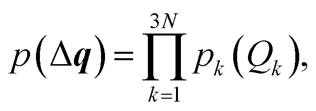23

and that the mean value corresponds to the undistorted structure, i.e., 〈Q_k〉 = 0. A generalization is usually possible by applying a suitable coordinate transformation.

The calculated spectrum will thus also become a random variable with an associated probability density,

24

The probability distribution for the calculated spectrum can be characterized by calculating its moments,

25

most importantly its mean 〈σ(E)〉 = m₁[σ(E)] and its variance Var[σ(E)] = m₂[σ(E)] − 〈σ(E)〉² or its standard deviation

For our surrogate model with up to two-mode contributions, the mean value of the probability distribution for the calculated spectrum can be calculated as,

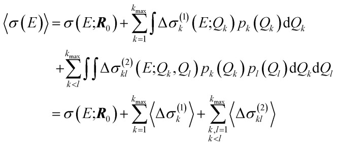26

Note that this mean value does not necessarily agree with the spectrum calculated for the undistorted structure, even tough the mean of the distribution of the distortions equals the reference structure.

If only one-mode contributions are included, the variance can be calculated as,

27

For surrogate models including two-mode contributions, explicit expressions are given in the ESI (Section S3).† More elaborate approaches (such as polynomial chaos expansions⁴⁷) for calculating the variance with higher-order surrogate models and for its analysis are available in the literature on uncertainty quantification (global sensitivity analysis).⁴⁸

For the test case of the XES spectrum of Fe(CO)₅, we assume a normal distribution with a mean of zero and with standard deviation s_Q for distortions along all sensitivity modes,

28

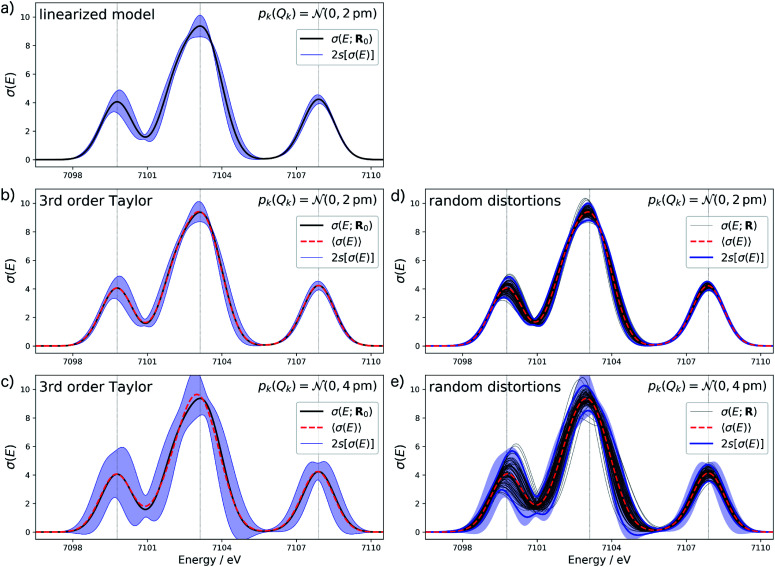
Thus, the probability that a distortions is within ±2s_Q is ca. 95%. In Fig. 4 we plot the error bars corresponding to two standard deviations s[σ(E)] for the calculated spectrum. Assuming the calculated spectra follow a normal distribution, the calculated spectra would lie within the error bars with a probability of 95%. Therefore, with s_Q = 2 pm in this setup we expect similar error bars as when considering maximum distortions of ±4 pm. Note, however, that because independent, normally-distributed distortions along all sensitivity modes are assumed, the expectation value of |ΔR| amounts to 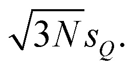Thus, the considered distortions are much larger than those considered above, but their largest part will always be along non-influential sensitivity modes.

Fig. 4. Calculated XES spectrum of Fe(CO)₅ (black line) including error bars (blue shaded area) corresponding to two standard deviations when assuming a normal distribution with standard deviation s_Q for the distortions of the underlying molecular structure. If different from the spectrum calculated for the reference structure, the mean of the calculated spectrum is included as dashed red line. (a) Error bars calculated for s_Q = 2 pm with the linearized surrogate model; (b and c) error bars calculated for (b) s_Q = 2 pm and (c) s_Q = 4 pm with the non-linear surrogate model based on a 3rd order Taylor expansion for the one-mode contributions and neglecting two-mode and higher-order contributions. (d and e) Spectra calculated for 100 random distortions sampled from independent normal distributions with (d) s_Q = 2 pm and (e) s_Q = 4 pm (black lines) as well as the error bars corresponding to two standard deviations (blue lines). For comparison, the error bars from (b) and (c), respectively, are included as blue shaded area.

The calculation of the error bars requires calculating the integrals in eqn (26) and (27). With our surrogate model based on a Taylor expansion of the one-mode contributions and normally distributed distortions these could be obtained analytically, but using a numerical integration scheme such as Gauss–Hermite quadrature or Monte–Carlo sampling is more general. For simplicity, here we apply numerical integration with a grid of 1000 evenly spaced points between −4s_Q and +4s_Q.

Fig. 4a shows the calculated XES spectrum of Fe(CO)₅ with 2s error bars assuming a normal distribution with 2s_Q = 4 pm for the structural distortions within the linearized surrogate model. In this case, the mean of the calculated spectrum coincides with the spectrum of the undistorted structure. Again, the error bars obtained with the linearized surrogate model show some unphysical features at the minimum at ca. 7101 eV and close to the maximum of the second peak at ca. 7103 eV. With the surrogate model employing a 3rd order Taylor expansion (see Fig. 4b) these mostly disappear and the error bars become overall smooth.

When increasing the standard deviation of the normal distribution assumed for the structural distortions to 2s_Q = 8 pm, the error bars increase (see Fig. 4c). However, this increase is not proportional and different new features are introduced for the individual peaks in the spectrum. For instance, the error bars for the second peak are larger for an increase in the intensity than for a decrease and also show a larger probability for a shift of this peak to lower energies. This also results in a shift of the mean of the calculated spectrum compared to the spectrum of the undistorted structure.

To verify the accuracy of the obtained error bars, we re-calculated the XES spectrum for 100 random distortions sampled from independent normal distributions for each Cartesian coordinate. These randomly sampled calculated spectra are shown in Fig. 4d and e for 2s_Q = 4 pm and 2s_Q = 8 pm, respectively, together with the corresponding error bars, obtained as two standard deviations of the calculated spectra. For 2s_Q = 4 pm (see Fig. 4d), we find an almost perfect agreement of the error bars obtained from random sampling with the error bars derived from our non-linear surrogate model. On the other hand, for 2s_Q = 8 pm (see Fig. 4e) larger deviations appear. For the first peak, the surrogate model predicts too large error bars at the low-energy shoulder of the peak, and for the third peak it overestimates the uncertainty for a shift of the peak position. These differences points to a breakdown of the 3rd order Taylor expansion for larger distortions. In addition, for larger distortions it is also not clear whether with only 100 random distortions, all relevant distortions are sampled sufficiently.

The main features of the error bars in Fig. 4 are overall similar to those already observed in Fig. 3. The largest error bars is found for the first and second peak, whereas the uncertainty is smaller for the third peak. To allow for a further analysis, Table 1 collects quantitative statistical metrics for the intensity at the positions of the three peaks. At the first and third peak, the mean on the calculated intensity 〈σ(E_j)〉 coincides with the intensity that is calculated for the undistorted structure σ(E_j;R₀), while for the second peak the mean intensity slightly deviates from the intensity for the reference structure. This deviation increases when increasing the standard deviation of the normal distribution that is assumed for the structural distortions.

Quantitative statistical metrics for the uncertainty of the calculated XES spectrum of Fe(CO)₅ at the maxima of the three considered peaks (E_j, indicated by vertical lines in the spectra in Fig. 4) assuming a normal distribution with standard deviation s_Q = 2 pm and s_Q = 4 pm for the distortions of the underlying molecular structure. Listed are the intensity for the undistorted structure σ(E_j;R₀), the mean of the intensity 〈σ(E_j)〉, its variance Var[σ(E_j)], its standard deviation s[σ(E_j)], and the coefficient of variance COV[σ(E_j)]. All metrics refer to the non-linear surrogate model based on a 3rd order Taylor expansion for the one-mode contributions and neglecting two-mode and higher-order contributions.

E j /eV	σ(Ej;R0)	〈σ(Ej)〉	Var[σ(Ej)]	s[σ(Ej)]	COV[σ(Ej)]
7099.8	4.06	4.06	0.16	0.40	0.10
7103.1	9.36	9.41	0.12	0.35	0.04
7107.9	4.23	4.23	0.02	0.15	0.04
7099.8	4.06	4.06	0.74	0.86	0.21
7103.1	9.36	9.54	0.47	0.69	0.07
7107.9	4.23	4.23	0.09	0.30	0.07

Table 1 further includes the variance of the intensity at the peak maxima Var[σ(E_j)], its standard deviation and the coefficient of variance (COV), s[σ(E_j)]/〈σ(E_j)〉. As it is normalized to the mean intensity, the latter gives a measure of the relative uncertainty. These quantitative metrics confirm the observations already made in Fig. 4, i.e., the absolute uncertainty, as measured by the variance or the standard deviation, is largest for the first and the second peak, while it is considerably lower for the third peak.

The COV shows that the relative uncertainty is the largest for the first peak, while it is considerably smaller for the second and third peak. When increasing the uncertainty that is assumed for the structural distortions by a factor of two, the standard deviation and COV approximately double for all three peaks. Note, however, that the considered metrics only account for the intensity at the position of the peak, and thus only partly capture differences in the uncertainty of the peak position.

5. Further test cases: XES, UV/Vis, and IR

The methodology for quantifying the structural sensitivity of calculated spectra developed in the previous sections is not restricted to the test case of the XES spectrum of Fe(CO)₅ considered so far, but should be generally applicable to different spectroscopies. To demonstrate this and to explore the limitations of the current approach, in this section we investigate additional test cases from XES, ultraviolet/visible (UV/Vis), and infrared (IR) spectroscopy. These test cases cover a divers set of computational spectroscopies treated with different computational approaches (ground-state ΔDFT, time-dependent DFT, and harmonic vibrational analysis).

First, we consider the XES spectrum of another iron complex, Fe(CO)₃(cod) (cod = cyclooctadienyl, C₈H₁₂).^39,49 This is another typical transition metal complex, but features a more complex coordination environment compared to Fe(CO)₅. The sensitivity of the calculated XES spectrum with respect to selected distortions has been explored previously in ref. 35. Here, we now consider distortions with respect to all possible distortions as described above.

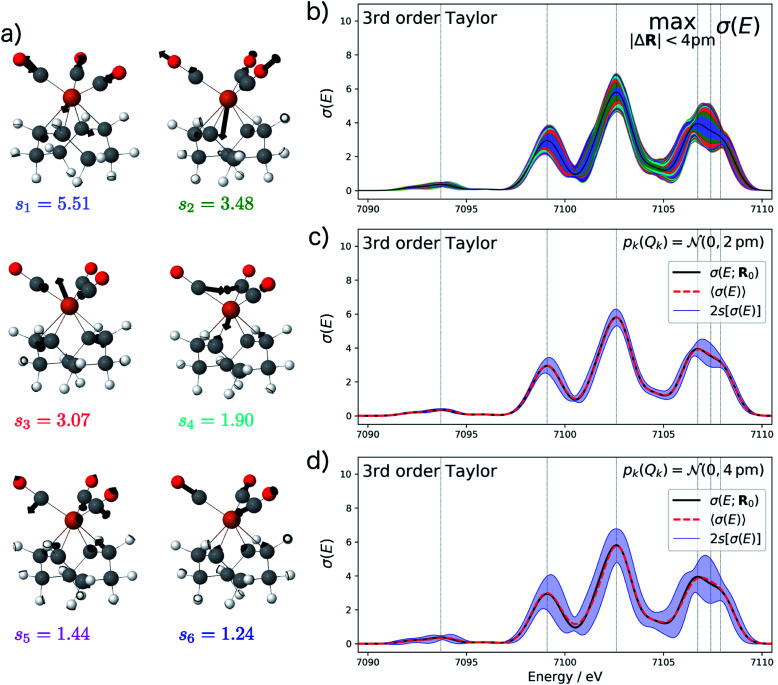
The sensitivity modes resulting from the principal component analysis are shown in Fig. 5a. We find that only 11 of the in total 81 sensitivity modes are required to account for 95% of the sum of all singular values. For these 11 sensitivity modes, we set up our surrogate model in the same fashion as for Fe(CO)₅, i.e., a 3rd order Taylor expansion was used for the one-mode contributions while neglecting two-mode and higher-order contributions. The calculated spectrum together with error bars is shown in Fig. 5b–d. A comparison to the error bars obtained from randomly sampling 100 distortions, which shows an excellent agreement with our non-linear surrogate model for both s_Q = 2 pm and s_Q = 4 pm, is given in Fig. S2 in the ESI.†

Fig. 5. Analysis of the structural sensitivity of the calculated XES spectrum of Fe(CO)₃(cod). (a) Visualization of the six most influential sensitivity modes. (b) Calculated spectrum including error bars giving upper and lower bounds for distortions with |ΔR| ≤ 4 pm. The colors of the shaded area indicate the contributions of the different sensitivity modes. (c and d) Calculated spectrum including error bars corresponding to two standard deviations when assuming a normal distribution with standard deviation (c) s_Q = 2 pm and (d) s_Q = 4 pm for the distortions of the molecular structure. All error bars are obtained using the non-linear surrogate model based on a 3rd order Taylor expansion for the one-mode contributions and neglecting two-mode and higher-order contributions.

As for Fe(CO)₅, the two most influential sensitivity modes correspond to C O stretching and Fe–C stretching vibrations. The third sensitivity mode can be interpreted as a Fe–cod stretching mode, whereas the fourth and fifth sensitivity mode describe deformations of the CO ligand sphere. Note that the most influential sensitivity modes do not include any changes of the structure of the cod ligand, which indicates that such distortions do not alter the calculated XES spectrum significantly.

The calculated error bars are similar to those found for Fe(CO)₅ for the three most intense peaks (see also Section S5 in the ESI† for a discussion of quantitative metrics). For the weak features between ca. 7092 and 7095 eV, the error bars are very small, i.e., even though it is only weak this region appears to be rather insensitive to structural distortions. Noteworthy are also the error bars for the third peak at ca. 7106–7109 eV. Within the error bars, this peak could show only one maximum (as for the reference structure) or two maxima. Such insights provided by the error bars for calculated spectra will potentially be crucial for the comparison of calculated and measured spectra.

As a second test case, we consider the electronic excitation (UV/Vis) spectrum of the dye molecule aminocoumarin C151. Such coumarin dyes are widely used for studying photochemistry and thus provide a typical test case. We have previously investigated aminocoumarin C151 as a model system for simulating solvent effects on electronic excitations.⁵⁰ Besides the effect of the solvent environment, a further contribution to such solvent effects are fluctuations of the molecular structure which have distinct effects on the calculated UV/Vis spectrum.

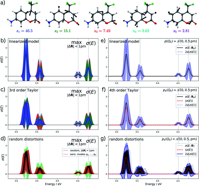
For analyzing the structural sensitivity of the calculated UV/Vis spectrum of aminocoumarin C151 we considered the region between 2.5 and 5.0 eV, in which four allowed electronic transitions are found. We performed a principal component analysis of the linear structural sensitivities as described above. Here, only five sensitivity modes, which are shown in Fig. 6a, are required to account for 95% of the sum of all 66 singular values. These all correspond to different ring breathing modes of the conjugated aromatic system. Note that the influence of the first sensitivity mode is already more than three times larger than for the second sensitivity mode.

Fig. 6. Analysis of the structural sensitivity of the calculated UV/Vis spectrum of aminocoumarin C151. (a) Visualization of the five most influential sensitivity modes. (b and c) Calculated spectrum including error bars giving upper and lower bounds for distortions with |ΔR| ≤ 1 pm obtained within (b) the linearized model and (c) the non-linear surrogate model based on a 4th order Taylor expansion for the one-mode contributions and neglecting two-mode and higher-order contributions. (d) Spectra calculated for 100 random distortions with |ΔR| = 1 pm (black lines) as well as 20 evenly spaced distortions between Q_i = ±1 pm along each of the four most influential sensitivity modes (red lines). The total error bars from (c) are included as green shaded area for comparison. (e and f) Calculated spectrum including error bars corresponding to two standard deviations when assuming a normal distribution with standard deviation s_Q = 0.5 pm for the distortions of the molecular structure obtain within (e) the linearized model and (f) the non-linear surrogate model. (g) Spectra calculated for 100 random distortions sampled from independent normal distributions with s_Q = 0.5 pm as well as the error bars corresponding to two standard deviations (blue lines). For comparison, the error bars from (f) are included as blue shaded area.

For the calculation of error bars, we used both the linearized model and a 4th order Taylor expansion of the one-mode contributions, while neglecting two-mode and higher-order contributions. The resulting error bars are shown in Fig. 6b, c, e and f. First, we notice that the effect of structural distortions on the calculated spectra is much larger than for XES. Therefore, we only consider maximum distortions of up to 1 pm and assumed a normal distribution with a standard deviation of s_Q = 0.5 pm, respectively. Even for these smaller distortions, the difference between the linearized model and the non-linear model using a 4th order Taylor expansion of the one-mode contributions is rather pronounced. With the linearized model, the error bars extend quite far to negative intensities, which is unphysical and indicates a breakdown of the linear approximation. This is to a large extent corrected when switching to a 4th order Taylor expansion.

Further inspection shows that for all peaks, the dominating effect of structural distortions is a shift of the peak position. Once this shift becomes large compared to the width of the peak, it is not well described by a linear expansion of the difference spectrum. This is most obvious in Fig. 6c for the first peak. Here, the 4th order Taylor expansion is mostly sufficient for recovering such a shift in the peak position (see Fig. 6d), but for larger shifts even a higher-order Taylor expansion might not be adequate. However, even though the 4th order Taylor expansion improves upon the linearized model, it still results in some unphysical extent of the calculated error bars to negative intensities. Note, that our form of the nonlinear surrogate model is also able to accommodate other approximations than a Taylor expansion for the one-mode (and possibly higher-order) contributions, which might be more suitable for describing larger shifts in peak positions.

To assess the accuracy of the error bars obtained with our nonlinear surrogate model, Fig. 6d and g show the spectra obtained for 100 randomly sampled distortions. For random distortions with |ΔR| = 1 pm (see Fig. 6d), all calculated spectra are within the boundaries for the maximum change in the calculated spectrum. However, the magnitude of the change is significantly smaller because the most influential distortions are not sampled sufficiently. When considering explicit distortions along the most influential sensitivity modes, the error bars are approached more closely. When sampling independent normally-distributed distortions (see Fig. 6g), we find that the error bars obtained from the standard deviation of the calculated spectra are in very good agreement with those obtained from the nonlinear surrogate model. Note that even though the spectra always remain positive, these error bars extend to negative intensities, which might appear unphysical. However, this is a consequence of the fact that the calculated spectrum do not follow a normal distribution anymore, which leads to a breakdown of the interpretation of the 2s error bars as 95% confidence intervals.

Finally, we consider the calculated harmonic IR spectrum of the amino acid alanine as a third test case. Vibrational spectroscopy is a prime example for a spectroscopic method that is used for making structural assignments based on the direct comparison of calculated and measured spectra (see, e.g., ref. 3–7). As many such studies concern polypeptides, alanine as one of the simplest amino acids is well suited as a first test case. Note that for vibrational spectra, the sensitivity of the calculated harmonic spectra with respect to structural distortions is related to the anharmonicity of the potential energy surface and the resulting error bars thus also give an indication for uncertainties resulting from the neglect of anharmonicities.

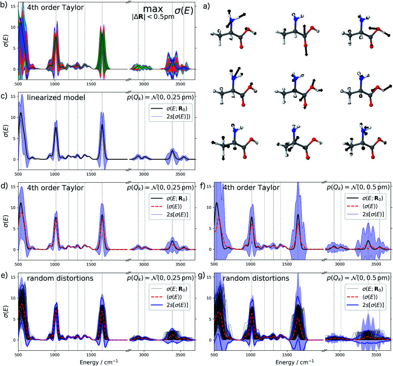
For the IR spectrum of alanine, we analyzed the structural sensitivity in the region between 500–4000 cm⁻¹. Here, we find that 13 out of 39 sensitivity modes need to be included to account for 95% of the sum of all singular values. The nine most influential sensitivity modes are visualized in Fig. 7a. The comparison with the color-coded error bars for maximum distortions of up to 0.5 pm in Fig. 7b shows that different peaks are affected by the individual sensitivity modes. For instance, the amide I (C O stretching) vibration at ca. 1650 cm⁻¹ is almost exclusively influenced by the second sensitivity mode, which corresponds to a change of the C O bond length.

Fig. 7. Analysis of the structural sensitivity of the calculated IR spectrum of alanine. (a) Visualization of the nine most influential sensitivity modes; (b) calculated spectrum including error bars giving upper and lower bounds for distortions with |ΔR| ≤ 0.5 pm. (c, d and f) Calculated spectrum including error bars corresponding to two standard deviations when assuming a normal distribution with standard deviation (c and d) s_Q = 0.25 pm and (f) s_Q = 0.5 pm for the distortions of the molecular structure. In (c) the error bars are obtained using the linearized model, while in (b), (d) and (f) a non-linear surrogate model is used that is based on a 4th order Taylor expansion for the one-mode contributions and neglecting two-mode and higher-order contributions. (e and g) Spectra calculated for 100 random distortions sampled from independent normal distributions with (e) s_Q = 0.25 pm and (g) s_Q = 0.5 pm as well as the error bars corresponding to two standard deviations (blue lines). For comparison, the error bars from (d) and (f), respectively, are included as blue shaded area.

As for UV/Vis spectroscopy, we find that also the calculated IR spectra are much more sensitive to structural distortions than the XES spectra. Therefore, we consider only normally distributed distortions with a standard deviation of s_Q = 0.25 pm in Fig. 7c and d. Again, we find that going from a linearized model to a 4th order Taylor expansion of the one-mode contributions significantly reduces the extent of the error bars to negative intensities. We also note that when going to normally distributed distortions with a standard deviation of s_Q = 0.5 pm (see Fig. 7f), the 4th order Taylor expansion breaks down, i.e., more sophisticated approximations for the one-mode contributions will be required for describing such larger distortions. This is confirmed by the comparison with the error bars obtained from randomly sampled distortions that is shown in Fig. 7e and g.

Inspecting the error bars in Fig. 7d as well as the corresponding quantitative statistical metrics listed in Table 2 reveals rather different uncertainties in different regions of the spectrum. While the fingerprint region below ca. 800 cm⁻¹ is subject to large absolute uncertainties as well as for the amide I peak at ca. 1650 cm⁻¹ (which mainly consists of the C O stretching vibration), a rather small absolute uncertainty is found for the position of the peak at ca. 1016 cm⁻¹ as well as for low-intensity peaks between ca. 1050 and 1500 cm⁻¹ (which are due to the C^α–N stretching, C^α–H bending and the symmetric CH₃ bending vibrations). In the high-wavenumber region, the C–H stretching vibrations in the region between ca. 2800–3150 cm⁻¹ is affected by a significantly smaller absolute uncertainty that the O–H and N–H stretching vibrations in the region between ca. 3200–3700 cm⁻¹.

Quantitative statistical metrics for the uncertainty of the calculated IR spectrum of alanine at the maxima of selected peaks (E_j, indicated by vertical lines in the spectra in Fig. 7). The statistical analysis assumes a normal distribution with standard deviation s_Q = 0.25 pm for the distortions of the underlying molecular structure. Listed are the intensity for the undistorted structure σ(E_j;R₀), the mean of the intensity 〈σ(E_j)〉, its variance Var[σ(E_j)], its standard deviation s[σ(E_j)], and the coefficient of variance COV[σ(E_j)]. All metrics refer to the non-linear surrogate model based on a 4th order Taylor expansion for the one-mode contributions and neglecting two-mode and higher-order contributions. See Table S11 in the ESI for the metrics for s_Q = 0.5 pm.

E j /cm−1	Assignment	σ(Ej;R0)	〈σ(Ej)〉	Var[σ(Ej)]	s[σ(Ej)]	COV[σ(Ej)]
534.7	Fingerprint	11.12	8.66	8.77	2.96	0.34
1015.6	X–H bend	7.70	7.22	0.48	0.69	0.10
1191.3	Cα–N stretch	0.88	0.86	0.00	0.04	0.05
1313.1	Cα–H bend	0.99	0.96	0.02	0.15	0.16
1412.5	Symm. CH3 bend	1.08	1.07	0.00	0.06	0.06
1650.9	C O stretch	8.31	7.18	3.52	1.88	0.26
2922.2	C–H stretch	0.79	0.66	0.05	0.22	0.34
3014.7	C–H stretch	0.59	0.54	0.02	0.13	0.24
3390.2	O–H stretch	2.07	1.10	0.88	0.94	0.85
3547.1	N–H stretch	0.58	0.37	0.05	0.23	0.62

Considering the COV, the latter stand out as the peaks with the highest relative uncertainty. For the C–H stretching, amide I (C O stretching), and the fingerprint region, the COV is smaller by about a factor of two, but is still sizable. The intensities of the peaks in the region between ca. 1050 and 1500 cm⁻¹ show not only the smallest absolute uncertainty, but also the smallest COV.

Such a systematic assessment of the uncertainties in the positions and intensities of different peaks in calculated vibrational spectra will potentially enable a much more reliable assignment of experimental spectra. Most importantly, it allows one to identify spectral features that are subject to high uncertainties. For these peaks, one can then selectively refine the computational methodology in order to reduce the uncertainty.

6. Conclusions and outlook

Altogether, we have presented a methodology for systematically quantifying the structural sensitivity of calculated molecular spectra. It allows for the inclusion of error bars indicating the uncertainties in a calculated spectrum that are due to uncertainties in the underlying molecular structure. It is thus a crucial first step towards theoretical spectroscopy with error bars and will enable a systematic assessment of the agreement between computational and experimental spectra. While we demonstrated its applicability to XES, UV/Vis, and IR spectroscopy, our methodology is not specific to certain spectroscopies but should be generally applicable to any type of computational spectroscopy providing a spectral intensity as function of excitation energy.

Our starting point for quantifying the structural sensitivity is a principal component analysis of the linear structural sensitivity with respect to all possible Cartesian displacements. This leads to sensitivity modes, which correspond to collective distortions of the reference structure. We could show that only a small fraction of all sensitivity modes need to be included to describe the full linear structural sensitivity. Currently, our approach initially requires the calculation of 6N spectra for displaced structures, which can be a significant increase of the computational effort. However, different strategies for making this step more efficient could be explored in future work, e.g., the analytical calculation of the derivative of the spectra with respect to structural distortions (see, e.g., ref. 51), the determination of the most influential sensitivity modes at a lower level of theory, or an iterative calculation of the largest singular values and the corresponding singular vectors.⁵²

Within the reduced space of the most influential sensitivity modes, one can subsequently set up a nonlinear surrogate model of the structural sensitivity, for which an HDMR expansion provides a convenient and general ansatz. Here, we employed a 3rd or 4th order Taylor expansion for the one-mode contributions and neglected two-mode and higher-order contributions. We found that such an approximation is sufficient as long as the shifts in peak positions remain small compared to their width. If this is no longer the case, more sophisticated approximations will be required, but can easily be accommodated within the general form of the surrogate model introduced here. For the systematic construction of surrogate models of the structural sensitivity, iterative schemes that include additional data points as needed could be devised in analogy to methods available for the construction of anharmonic potential energy surfaces.^53,54

With a surrogate model of the structural sensitivity, it becomes possible to perform a statistical analysis of the propagation of uncertainties in the molecular structure to the calculated spectra, which ultimately provides error bars for the calculated spectra. In the present work, we assumed an ad hoc uncertainty for the molecular structure, either by specifying a maximum distortion or by assuming a normal distribution with a certain standard deviation. In future applications, these structural uncertainties could be obtained from more physical considerations, e.g., by assuming a thermal population of vibrational modes. Here, we characterized the uncertainty in the calculated spectrum either by giving upper and lower bounds or by calculating the standard deviation of the probability distribution for the calculated spectra. This could be extended by performing additional statistical analyses, e.g., by explicitly calculating confidence or credible intervals for the calculated spectrum.

The resulting error bars make it possible to identify which spectral features are associated with a large structural sensitivity and which spectral features are rather insensitive to distortions of the underlying molecular structure. For instance, our analysis of the structural sensitivity of the calculated IR spectrum of alanine reveals that peaks that are due to stretching modes show a significantly larger uncertainty than those due to bending modes. Moreover, the analysis of the sensitivity modes reveals the collective distortions that have the largest influence on the calculated spectrum. For alanine, we find that changes of the N–H, O–H, and C O bond lengths have the largest effect on the calculated IR spectrum. Altogether, the novel analysis tools developed here make it possible to assess the relationship between molecular structure and calculated spectra in a quantitative way and will ultimately make structural assignments based on the comparison of experimental and calculated spectra more reliable.

Here, we have considered distortions of the underlying molecular structure as the only source of uncertainty. Of course, calculated spectra are also subject to additional sources of uncertainty, most importantly errors of the approximate exchange–correlation functional in DFT. The methodology presented here can be combined with existing approaches for quantifying such uncertainties of quantum-chemical approximations (see e.g., ref. 23–27). Moreover, our general methodology can be extended to other sources of uncertainties that depend on a larger number of parameters, e.g., uncertainties introduced by an environment that is described by an embedding potential.⁵⁵ Ultimately, we envision the quantification of all relevant sources of uncertainties in calculated spectra, and consider the present work an important step in this direction.

Appendix: computational details

All quantum-chemical calculations have been performed using the Amsterdam Density Functional (ADF) program package.^56,57 The calculations were automated using the PyADF scripting framework,⁵⁸ and the methodology for the analysis of the structural sensitivity of calculated spectra described here has been implemented as an add-on to PyADF. Normally-distributed random distortions (used in Fig. 4d, e, 6g, 7e and g) are obtained by drawing each component of the displacement vector ΔR from an independent normal distribution with the desired standard deviation. Random distortions with a given magnitude |ΔR| (used in Fig. 3c and 6d) are obtained from these normally-distributed random distortions by rescaling the displacement vector accordingly.

The molecular structures of Fe(CO)₅ and of Fe(CO)₃(cod) were optimized employing the BP86 exchange–correlation (xc) functional^59,60 in combination with a Slater-type TZ2P basis set.⁶¹ For aminocoumarin C151, the structure was optimized using BP86 and a TZP basis set. For alanine, BP86 and a DZ basis set were used in combination with a COSMO solvation model⁶² with default parameters.

For the calculation of XES spectra, we employed the ΔDFT approach of Lee et al.,³⁸ in which excitation energies are calculated as occupied orbital energy differences. This ΔDFT approach is a rather simple approximation, but it has been shown to be reliable for valence-to-core XES spectra of diverse transition metal complexes,^63–71 including the ones considered here.³⁹ XES intensities are obtained from transition moments between occupied orbitals, including contributions beyond the electric dipole approximation.^72,73 All calculations of XES spectra were performed with the BP86 xc functional and a QZ4P basis set in combination with the COSMO solvation model⁶² with default parameters. The calculated spectra were shifted by 180.62 eV (ref. 35 and 49) and a Gaussian line broadening with a full-width at half maximum of 1.5 eV was applied to each calculated transition. For Fe(CO)₅, we considered the region between 7094.62 eV and 7110.62 eV as relevant energy range, whereas for Fe(CO)₃(cod) the region between 7088.62 eV and 7110.62 eV was used.

The UV/Vis spectrum of aminocoumarin C151 was calculated using time-dependent DFT (TD-DFT) as implemented in ADF.⁷⁴ In all TD-DFT calculations, the SAOP model potential^75,76 was used in combination with a TZP basis set. The spectra were obtained by applying a Gaussian line broadening with a FWHM of 0.08 eV, and the broadened spectrum in the region between 2.5 eV and 5.0 eV was used as quantity of interest.

Harmonic infrared spectra of alanine were calculated with ADF using its analytical frequency module⁷⁷ using BP86/DZ and a COSMO solvation model. A Gaussian line broadening with a FWHM of 50 cm⁻¹ was employed. Here, the broadened spectrum was considered in the region between 500 cm⁻¹ and 4000 cm⁻¹.

Author contributions

CRJ designed the study and supervised the project. TGB and MOW developed the methodology and algorithms. TGB implemented the software, assisted by MOW. TGB performed all calculations and wrote a first draft of the manuscript. CRJ wrote the final version of the manuscript, which all authors critically revised and approved.

Conflicts of interest

There are no conflicts to declare.