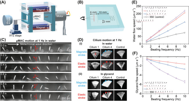
Figure 3.
Metachronal μMAC motion in a 2D rotating uniform magnetic field and the fluid pumping capability. (A) Schematic diagram of the magnetic actuation setup for creating a 2D rotating magnetic field. The details of the generated magnetic field are available in Figure S2. Illustration is not to scale. (B) Schematic drawing of the square microfluidic chip including the μMAC, indicating the observation area of the generated flow. Illustration is not to scale. (C) Snapshots of the metachronal motion of one row of μMAC with a pitch of 550 μm during one beating cycle at 1 Hz in water (see Movie S3). The electric motor rotates counterclockwise. The white arrow indicates the traveling direction of the metachronal wave. The red arrows indicate the direction of the applied magnetic field. The encircled numbers indicate the sequence of the μMAC for reference in later analyses. (D) Side-view time-lapse images of cilium motion at 1 Hz in both water and glycerol, showing a 2D symmetric motion. β represents the opening angle of the cilium motion. The blue dashed line and the red dashed line indicate the tip trajectory during the magnetic stroke and elastic stroke, respectively. The motion of cilium 4 during the elastic stroke in both water and glycerol is available in Movie S6. The motion of the whole μMAC array in both water and glycerol can be found in Figure S3. Note the difference in the recording speed for the metachronal μMAC and the control μMAC, as well as for in water and in glycerol. See Experimental Section for details. (E,F) Generated flow speed of water (E) and glycerol (F) as a function of the beating frequency of the metachronal μMAC array with pitches of 350, 450, and 550 μm, respectively, as well as the control μMAC array with a pitch of 550 μm. A positive result represents a flow above the ciliated area in the same direction as the metachronal wave traveling direction. The trajectories of the tracer particles in both water and glycerol can be found in Figure S4. The corresponding volumetric flow rate and pressure drop are available in Figure S5. Each data point was obtained by averaging the results of at least ten measurements.

