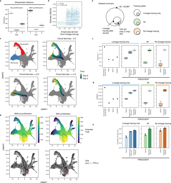
Fig. 2. Fate outcomes generated by PRESCIENT align with experimental lineage tracing when taking into account cell proliferation.

a Testing performance of models trained with and without proliferation on the task of recovering the held-out time point, day 4. Performance is reported as Wasserstein distance of simulated population with respect to actual populations at the given time points for models trained without and with proliferation over n = 5 seeds. Dashed line indicates distance of linearly interpolated population with respect to the actual population on day 4. b Correlation of actual and estimated proliferation rates on day 2 cells with lineage tracing data (n = 4638). c Examples of n = 50 trajectories with starting cells assigned different clonal fate biases. The color-scale indicates time corresponding to 100 time steps of dt = 0.1 starting from t = 2. Clonal fate bias is computed with respect to monocyte/neutrophil populations at the final time point. d Visualizations of underlying potential and drift functions learned by models with and without cell proliferation. Drift is visualized for a random sample of cells. Dotted circle indicates qualitative differences in potential landscape. e Summary of training/test splits of lineage tracing dataset. Training sets either include only cells with lineage tracing data, all cells, or cells without lineage tracing data. f–h, Performance of other methods (far left, Smoothed fate probabilities given by held-out clonal data, PBA: population balance analysis¹⁰, WOT: Waddington-OT⁸, FateID⁹ evaluated using predictions provided by Weinreb et al.) in comparison to PRESCIENT (left-right) on predicting clonal fate bias for the same test set (n = 335) given different training sets. Training sets either consisted of only cells for which lineage tracing data was available (left), all cells (middle), or cells without lineage tracing data (right). Performance metrics evaluated include f Pearson r, g AUROC, and h fraction of test set in which at least 1 simulated cell at the final time point is either classified as a neutrophil or a monocyte over n = 5 seeds. In b, f–g, boxplots indicate median (middle line), first and third quartiles (box), and the upper whisker extends from the edges to the largest value no further than 1.5 × IQR (interquartile range) from the quartiles and the lower whisker extends from the edge to the smallest value at most 1.5 × IQR of the edge, while data beyond the end of the whiskers are outlying points that are plotted individually as diamonds. In h, bar plots show the average fraction of cells with error bars representing the 95% CI.