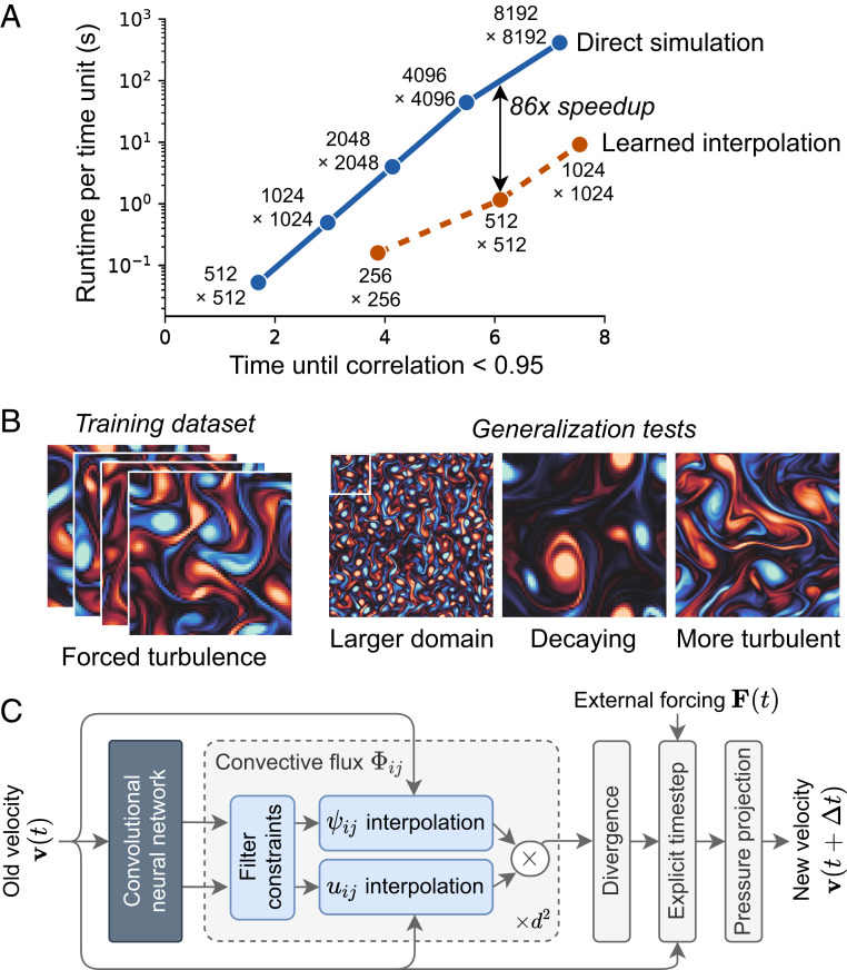
Fig. 1.

Overview of our approach and results. (A) Accuracy versus computational cost with our baseline (direct simulation) and ML-accelerated [learned interpolation (LI)] solvers. The $x$ axis corresponds to pointwise accuracy, showing how long the simulation is highly correlated with the ground truth, whereas the $y$ axis shows the computational time needed to carry out one simulation time unit on a single Tensor Processing Unit (TPU) core. Each point is annotated by the size of the corresponding spatial grid; for details see SI Appendix. (B) Illustrative training and validation examples, showing the strong generalization capabilities of our model. (C) Structure of a single time step for our LI model, with a convolutional neural net controlling learned approximations inside the convection calculation of a standard numerical solver. $\psi$ and $u$ refer to advected and advecting velocity components. For $d$ spatial dimensions there are $d^2$ replicates of the convective flux module, corresponding to the flux of each velocity component in each spatial direction.