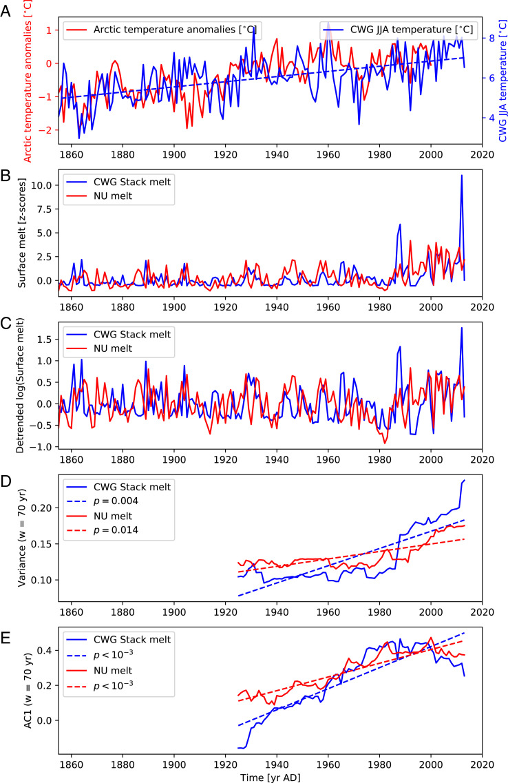
Fig. 1.

(A) Summer sea level temperatures from the Ilulissat station in CWG (25) (blue curves) and Arctic temperature anomalies (26) (red curves). The linear trend of the station data (dashed blue curve) corresponds to $1.3\hspace{0.17em}°$C warming per century. Arctic temperature anomalies are shown only for comparison; only the station data (blue curves) are used for our analysis. (B) Melt rates from the CWG ice core stack (blue curve) and the NU peninsula core (red curve), given as z scores with respect to a normal distribution (18). (C) Detrended logarithmic CWG (blue curve) and NU (red curve) melt rates. A Gaussian filter with bandwidth $\sigma =30$ y was used for detrending. The runoff and melt time series are preprocessed in this way before computing the EWS indicators to exclude potential biases by underlying trends; in particular, we take the logarithm of the melt rates in order to account for skewed data distributions. (D) The variance of the CWG (blue curves) and NU (red curves) melt rates. (E) The AC1 of the CWG (blue curves) and NU (red curves) melt rates. Note that the AC1, despite a significantly positive trend, appears to have at least temporarily stabilized in the last few decades. It should be noted, however, that the AC1 is generally influenced by (multi)decadal variability (27). The window size for computing the variance and the AC1 is $w=70$ y, and values are plotted at the windows’ endpoints. Data for the first $w=70$ y are omitted to ensure that all windows contain the same number of data points. The dashed lines in D and E indicate linear trends of the variance and AC1, and P values for positive slopes as determined from a phase surrogate test are indicated in the legend (see Materials and Methods). The statistical significance of the positive trends is robust across wide ranges of the bandwidth $\sigma$ and the sliding window size (SI Appendix, Fig. S1).