Deep collaborative learning with application to multimodal brain development study

Abstract

Multi-modal fMRI imaging has been used to study brain development such as the difference of functional connectivities (FCs) between different ages. Canonical correlation analysis (CCA) has been used to find correlations between multiple imaging modalities. However, it is unrelated to phenotypes. On the other hand, regression models can identify phenotype related imaging features but overlook the cross-modal data correlation. Collaborative regression (CR) is thus introduced to incorporate correlation as a penalization term into the regression model. Nevertheless, the complex relationship (e.g., nonlinear predictive relationship) between multiple data yet cannot be captured using linear CR models. To this end, we propose a novel method, deep collaborative learning (DCL), to address their limitations. DCL first uses a deep network to represent original data and then seeks their correlations, while also linking the data representation with phenotypical information. Therefore, DCL can better combine complex correlations between multiple data sets in addition to their fitting to phenotypes, with the potential to overcome the limitations of several current models. Based on DCL model, we study the difference of FCs between different age groups and also use FCs as a fingerprint to predict cognitive abilities. Our experiments demonstrated higher accuracy of using DCL over other conventional models when classifying populations of different ages and cognitive scores. Moreover, our experiments showed that different age or cognition groups may exhibit more significant differences of FCs in several networks than others. Furthermore, DCL revealed that brain connections became stronger at adolescence stage, demonstrating the importance of adolescence for brain development. In addition, DCL detected strong correlations between default mode network (DMN) and other networks which were overlooked by linear CCA, demonstrating DCL’s ability of detecting nonlinear correlations.

I. Introduction

BRAIN connectivity depicts the functional relations between different brain regions or networks [1]. Different brain regions function and harmonize in a connected network when performing a specific brain function [2]. Therefore, studying the connections of different brain sub-networks may help understand the functional mechanism of the brain and the change of brain connectivity may be a cause of mental disorders. Investigating changes in brain functional connectivity (FC) has been increasingly studied in recent years [3], [4]. An assumption is that adolescence (age 8-22) is an important stage for brain development and brain FC becomes more established around age 12 [5]. A number of studies [6], [7] have investigated how brain FC changes during adolescence and how it differs between different age groups, e.g., children and young adults, which further contribute to the study of normal and pathological brain development. The studies of brain FC have been focused on two aspects: to directly compare the difference of FC between different age groups and to use brain FC as features for age classification, which in return demonstrate the significant difference of FC between age groups. Brain FC have been shown to be discriminative regarding age group classification and studies [8], [9] even utilized brain FC as finger-prints to identify individuals.

Recent advances in functional magnetic resonance imaging (fMRI), have facilitated the production of multiple data for brain FC study. The brain FCs from different fMRI modalities, e.g. resting state fMRI (rs-fMRI) and task state fMRI (t-fMRI), may have common connections [10] and the fusion of multi-fMRI data can lead to a better understanding of the brain. A number of statistical learning models, e.g., canonical correlation analysis (CCA) [11], parallel independent component analysis (ICA) [12], deep neural networks [13], have been used to integrate multiple brain imaging data to study the interactions between different brain regions as well as the interactions between functional connectivity (FC) and genetic factors. Among these, CCA has been widely used to detect multivariate correlations for multi-modal and imaging genetics studies. Similar to principal component analysis (PCA), CCA is also a method for dimension reduction and data representation which projects original data into lower dimensional spaces. However, without additional processing steps, canonical variables lack phenotype related information which may restrict the application of CCA and the interpretation of its results. To address the limitation of CCA, Gross et al. [14] proposed a new model, called collaborative regression, which incorporated a regression penalty into CCA so that the model can identify correlations with discriminative power for phenotypes. As a result, the representation retains information relevant to both phenotypes and correlation. However, according to the simulation experiments in [14], collaborative regression may result in poor performance for prediction. This may be due to its formulation, in which both the correlation and the prediction projection variables are restricted to be the same. Moreover, the complex nonlinear relationship between multiple data types is another challenge for linear collaborative regression model to capture.

In this paper, we propose a novel model, deep collaborative learning (DCL) for multimodal data integration, which uses deep networks to represent multiple data sets while incorporating their correlations. The use of deep networks in the model enable it to be more flexible in representing complex/nonlinear information in the data. Our application to brain imaging studies verified the superior performance of the DCL model over several baseline classifiers, which results in lower prediction errors with multiple data sets while detecting their correlations. Many interesting findings were also discovered when DCL was applied to the brain connectivity study, as presented in the results section.

The rest of the paper is organized as follows. Section II describes the limitations of several existing multi-modal fusion methods and how the proposed model addresses the limitations. Data collection and preprocessing procedures as well as experiments and results of applying DCL to brain connectivity study can be found in Section III. Detailed discussions and analysis of the results were in Section IV. The discussion and conclusion of the work were given in Section IV.

II. Method

A. Overview of canonical correlation analysis (CCA)

Canonical correlation analysis (CCA) [15] is a model widely used for analyzing linear correlations between two data. It provides a way to study complex diseases using multi-omics data by investigating their cross-covariances.

Specifically, given two data matrices $X_1\in {\mathbb{R}}^{n\times r}$, $X_2\in {\mathbb{R}}^{n\times s}$ (n represents sample/subject size, and r, s represents the feature/variable sizes in two data sets), CCA seeks two coefficient vectors $u_1\in {\mathbb{R}}^{r\times 1}$ and $u_2\in {\mathbb{R}}^{s\times 1}$ by optimizing the Pearson correlation between X₁u₁ and X₂u₂, as in Eq. 1.

$$(u_1^{\ast },u_2^{\ast })=\underset{u_1,u_2}{\text{argmax}}{u}_1^{\prime }{\Sigma }_{12}{u}_2$$ (1)

subject to $u_1^{\prime }{\Sigma }_{11}{u}_1=1$, $u_2^{\prime }{\Sigma }_{22}{u}_2=1$ where $u_1\in {\mathbb{R}}^{r\times 1}$, $u_2\in {\mathbb{R}}^{s\times 1}$, ${\Sigma }_{ij}≔X_i^{\prime }{X}_j$

The identified canonical vectors $X_1{u}_1,X_2{u}_2\in {\mathbb{R}}^{n\times 1}$ are linear combinations of raw features/variables in original data X₁, X₂, which can facilitate multi-omics association interpretation due to the reduced dimension. Due to the constraints in Eq. 1, $u_1^{\prime }{\Sigma }_{12}{u}_2$ equals the cross-data correlation, i.e., $u_1^{\prime }{\Sigma }_{12}{u}_2=\frac{u_1^{\prime }{\Sigma }_{12}{u}_2}{\sqrt{u_1^{\prime }{\Sigma }_{11}{u}_1{u}_2^{\prime }{\Sigma }_{22}{u}_2}}$.

CCA can detect a series of canonical vectors that are pair-wise independent and guarantee the highest total correlation, as shown in Eq. 2.

$$(U_1^{\ast },U_2^{\ast })=\underset{U_1,U_2}{\text{argmax}}\text{Trace}(U_1^{\prime }{\Sigma }_{12}{U}_2)$$ (2)

subject to $U_1^{\prime }{\Sigma }_{11}{U}_1=U_2^{\prime }{\Sigma }_{22}{U}_2={\mathbf{I}}_n$; where $U_1\in {\mathbb{R}}^{r\times k}$,$U_2\in {\mathbb{R}}^{s\times k},k=\text{min}(\text{rank}(X_1),\text{rank}(X_2))$

As Σ₁₁, Σ₂₂ may be singular but the computation of ${\Sigma }_{11}^{-1}$, ${\Sigma }_{22}^{-1}$ is necessary when calculating loading vectors, matrix regularization is usually performed on Σ₁₁, Σ₂₂ as follows to ensure that Σ₁₁, Σ₂₂ are positive definite

$$\begin{gathered} {\widehat{\Sigma }}_{11}={\Sigma }_{11}+r_1{\mathrm{I}}_r \\ {\widehat{\Sigma }}_{22}={\Sigma }_{22}+r_2{\mathrm{I}}_s \end{gathered}$$ (3)

B. Collaborative regression (CR)

CCA is a method of data representation or dimension reduction. However, in the representation of CCA, canonical variables, are not phenotype/label related; this is in contrast with the widely used PCA that retains label related information in its representation. To address the limitation of CCA’s representation, Gross et al. [14] proposed a novel model, called collaborative regression, whose formulation is shown in Eq. 4. Given phenotype data $Y\in {\mathbb{R}}^{n\times 1}$, collaborative regression maximizes the following objective function

$$\begin{gathered} (u_1^{\ast },u_2^{\ast })=\underset{u_1,u_2}{\text{argmin}}{b}_1\Vert X_2{u}_2-X_1{u}_1{\Vert }_2 \\ +b_2\Vert Y-X_1{u}_1{\Vert }_2+b_3\Vert Y-X_2{u}_2{\Vert }_2 \end{gathered}$$ (4)

Collaborative regression addresses the limitations of CCA by incorporating a regression penalty into CCA so that the model can identify correlations with discriminative power for a particular phenotype. Therefore, the representation retains both phenotypes related and cross-data relationship information. However, when used for classification, collaborative regression did not produce higher classification accuracy compared to that of using regression and LASSO [16], according to the simulation experiments in [14]. Collaborative regression uses the same set of variables to represent both the regression and correlation, demanding for best fitting of phenotypes with multiple data sets while incorporating their correlations. Despite the success of collaborative regression, a linear relationship is assumed in the model, rendering it difficult to capture complex relationship between data sets.

C. Deep CCA

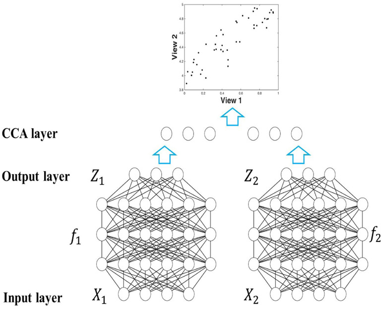
CCA may face another limitation in that it can only capture linear correlations and cannot detect complex nonlinear correlations. To address this problem, Deep CCA was proposed by Andrew et al. [17] to detect nonlinear correlations. As illustrated in Fig. 1, deep CCA introduces a deep network representation before applying CCA framework. Unlike linear CCA, which seeks the optimal canonical vectors U₁, U₂, deep CCA seeks the optimal network representation f₁(X₁), f₂(X₂), as shown in Eq. 5.

$$(f_1^{\ast },f_2^{\ast })=\underset{f_1,f_2}{\text{argmax}}\left\{\underset{U_1,U_2}{\max }\frac{U_1^{\prime }{f}_1(X_1)f_2(X_2)U_2}{\Vert f_1(X_1)U_1{\Vert }_2\Vert f_2(X_2)U_2{\Vert }_2}\right\}$$ (5)

where f₁, f₂ are two deep networks as illustrated in Fig. 1.

Fig. 1:

The work-flow of deep CCA. Data X₁, X₂ are input; deep networks f₁, f₂ work on X₁, X₂ and yield Z₁, Z₂ as output, to which CCA is applied subsequently. The optimization problem is to find the optimal network ${\widehat{f}}_1$, ${\widehat{f}}_2$ with the highest canonical correlation.

The introduction of deep network representation leads to a more flexible way to detect both linear and nonlinear correlations. According to experiments on both speech data and handwritten digits data [17], deep CCA’s representation was more effective in finding correlations than other methods, e.g., linear CCA, and kernel CCA. It was also shown in the work of [18] that both deep CCA and its extended version, deep canonically correlated auto-encoders, performed better in terms of both clustering and classification than other methods, e.g., linear CCA, kernel CCA. Despite the superior performance of deep CCA in detecting complex correlations, it still lacks phenotype related information.

D. Deep collaborative learning (DCL)

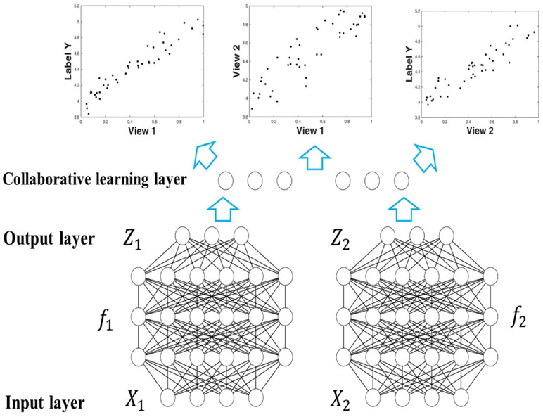
To address the limitations of both CCA and collaborative regression method, we propose a novel model, deep collaborative learning (DCL), which seeks a deep network representation of two data sets while incorporating their correlations into the model at the same time. Assume we have two modality data $X_1\in {\mathbb{R}}^{n\times r}$, $X_2\in {\mathbb{R}}^{n\times s}$ and a phenotype or label data $Y\in {\mathbb{R}}^{n\times 1}$, where n denotes sample size (number of subjects) and r, s are the dimensionality of feature of X₁, X₂ respectively. The formulation of deep collaborative learning is shown in Eqs. 6 and 7 and its work-flow is illustrated in Fig. 2.

$$\begin{gathered} (Z_1^{\ast },Z_2^{\ast })=\underset{Z_1,Z_2}{\text{argmax}}\{\underset{U_1,U_2}{\max }\text{Trace}(U_1^{\prime }{Z}_1^{\prime }{Z}_2{U}_2)- \\ \underset{{\beta }_1}{\text{min}}\Vert Y-Z_1{\beta }_1{\Vert }_2^2-\underset{{\beta }_2}{\text{min}}\Vert Y-Z_2{\beta }_2{\Vert }_2^2\} \end{gathered}$$ (6)

$$\begin{gathered} =\underset{Z_1,Z_2}{\text{argmax}}\{\Vert {\Sigma }_{11}^{-\frac{1}{2}}{\Sigma }_{12}{\Sigma }_{22}^{-\frac{1}{2}}\Vert tr \\ -\Vert Y-Z_1(Z_1^{\prime }{Z}_1{)}^{-1}{Z}_1^{\prime }Y{\Vert }_2^2 \\ -\Vert Y-Z_2(Z_2^{\prime }{Z}_2{)}^{-1}{Z}_2^{\prime }Y{\Vert }_2^2\} \end{gathered}$$ (7)

$$=\underset{Z_1,Z_2}{\text{argmax}}F(Z_1,Z_2)$$ (8)

where $Z_1=f_1(X_1)\in {\mathbb{R}}^{n\times p}$, $Z_2=f_2(X_2)\in {\mathbb{R}}^{n\times q}$, f₁, f₂ are two deep networks as illustrated in Fig. 2, ${\Sigma }_{ij}≔Z_i^{\prime }{Z}_j$, and $\Vert A{\Vert }_{tr}≔\text{Trace}(\sqrt{A^{\prime }A})=\Sigma {\sigma }_i$; U₁, U₂ in Eq. 6 subject to $U_1^{\prime }{\Sigma }_{11}{U}_1=U_2^{\prime }{\Sigma }_{22}{U}_2=\mathbf{I}$ As shown in Eqs. 6 and 7, deep collaborative learning seeks the optimal network representation Z₁ = f₁(X₁), Z₂ = f₂(X₂). In comparison, linear CCA and linear collaborative regression seek the optimal projection vectors u₁, u₂, as shown in Eqs. 1, 4. Compared to linear CCA and deep CCA, DCL’s representation retains label related information for better data fitting. Moreover, unlike linear collaborative regression, DCL uses a deep network representation, resulting in better detection of nonlinear relationships in the data while fitting to the phenotypes. In particular, DCL relax the requirement of linear collaborative regression model that the projection, u₁, u₂, have to be in the same direction. This can result in a better representation of both phenotypical information and cross-data correlation in an effective manner.

Fig. 2:

The work-flow of deep collaborative learning. Data X₁, X₂ are the input; deep networks f₁, f₂ operate on X₁, X₂ and yield Z₁, Z₂ as the output, to which collaborative learning is applied subsequently. Collaborative learning layer connects the two deep networks and passes two composite gradients mutually during the back-propagation process. The optimization problem is to find the optimal network ${\widehat{f}}_1$, ${\widehat{f}}_2$ which give both the highest canonical correlation and the lowest prediction error regarding label data Y.

For the purpose of computational efficiency, we use a first order optimization method, mini-batch stochastic gradient descent (mini-batch SGD), to solve the optimization problem. Back-propagation (BP) algorithm is used to pass the gradient backward to each layer of the network during each iteration step. In addition, dropout technique is used to avoid overfitting. In order to apply SGD and BP, we need to calculate the gradient of DCL’s objective function 7.

The gradient of objective function 7 is

$$\begin{gathered} \frac{\partial F(Z_1,Z_2)}{\partial Z_1}=-Z_1{\Sigma }_{11}^{-\frac{1}{2}}UD{U}^{\prime }{\Sigma }_{11}^{-\frac{1}{2}} \\ +Z_2{\Sigma }_{22}^{-\frac{1}{2}}V{U}^{\prime }{\Sigma }_{11}^{-\frac{1}{2}}+2Y{Y}^{\prime }{Z}_1(Z_1^{\prime }{Z}_1{)}^{-1} \\ -2Z_1(Z_1^{\prime }{Z}_1{)}^{-1}{Z}_1^{\prime }Y{Y}^{\prime }{Z}_1(Z_1^{\prime }{Z}_1{)}^{-1} \end{gathered}$$ (9)

$$\begin{gathered} \frac{\partial F(Z_1,Z_2)}{\partial Z_2}=-Z_2{\Sigma }_{22}^{-\frac{1}{2}}VD{V}^{\prime }{\Sigma }_{22}^{-\frac{1}{2}} \\ +Z_1{\Sigma }_{11}^{-\frac{1}{2}}U{V}^{\prime }{\Sigma }_{22}^{-\frac{1}{2}}+2Y{Y}^{\prime }{Z}_2(Z_2^{\prime }{Z}_2{)}^{-1} \\ -2Z_2(Z_2^{\prime }{Z}_2{)}^{-1}{Z}_2^{\prime }Y{Y}^{\prime }{Z}_2(Z_2^{\prime }{Z}_2{)}^{-1} \end{gathered}$$ (10)

where $[U,D,V]=\text{svd}({\Sigma }_{11}^{-\frac{1}{2}}{\Sigma }_{12}{\Sigma }_{22}^{-\frac{1}{2}})$

To prove 9, we showed

$$\begin{gathered} \frac{\partial \Vert Y-Z_1(Z_1^{\prime }{Z}_1{)}^{-1}{Z}_1^{\prime }Y{\Vert }_2^2}{\partial Z_1}=2Y{Y}^{\prime }{Z}_1(Z_1^{\prime }{Z}_1{)}^{-1} \\ -2Z_1(Z_1^{\prime }{Z}_1{)}^{-1}{Z}_1^{\prime }Y{Y}^{\prime }{Z}_1(Z_1^{\prime }{Z}_1{)}^{-1} \end{gathered}$$ (11)

and

$$\begin{gathered} \frac{\partial }{\partial Z_1}\Vert {\Sigma }_{11}^{-\frac{1}{2}}{\Sigma }_{12}{\Sigma }_{22}^{-\frac{1}{2}}{\Vert }_{tr}=-Z_1{\Sigma }_{11}^{-\frac{1}{2}}UD{U}^{\prime }{\Sigma }_{11}^{-\frac{1}{2}} \\ +Z_2{\Sigma }_{22}^{-\frac{1}{2}}V{U}^{\prime }{\Sigma }_{11}^{-\frac{1}{2}} \end{gathered}$$ (12)

The detailed derivation of the gradient can be found in Appendix.

E. Significance test for correlation analysis

Bartlett’s test [19], [20] is used to evaluate the significance of the canonical correlations of DCL’s outputs. A statistic for evaluating the significance of canonical correlations is

$$\Lambda ≔\prod _{i=1}^k(1-{\sigma }_i^2)$$ (13)

The distribution of Eq. 13 can be easily computed with Fisher transform $z≔\frac{1}{2}\log \left(\frac{1+{\sigma }_i}{1-{\sigma }_i}\right)$ when k = 1, and a similar distribution can be derived when k = 2 [20]. However, the exact distribution of Λ is not known when k > 2. Bartlett [20] provided a statistic which approximately follows a χ² distribution with freedom of p × q as in Eq. 14

$$\begin{gathered} {\chi }^2=-((n-1)-\frac{p+q+1}{2})\log \prod _{i=1}^k(1-{\sigma }_i^2) \\ \sim {\chi }^2(pq). \end{gathered}$$ (14)

Algorithm 1 Algorithm for deep collaborative learning

$$\begin{array}{cc}\hfill & 1:\mathrm{Input}{X}_1\in {\mathbb{R}}^{n\times r},X_2\in {\mathbb{R}}^{n\times s},\text{label}Y\in {\mathbb{R}}^{n\times 1},\text{initial}\hfill \\ \hfill & \text{networks}{f}_1^0,f_2^0\hfill \\ \hfill & 2:\mathrm{Output}\text{Optimal networks}{\widehat{f}}_1,{\widehat{f}}_2\text{with}{\widehat{Z}}_1={\widehat{f}}_1(X_1)\in \hfill \\ \hfill & {\mathbb{R}}^{n\times p},{\widehat{Z}}_2={\widehat{f}}_2(X_2)\in {\mathbb{R}}^{n\times q}\hfill \\ \hfill & 3:{\widehat{Z}}_1\leftarrow f_1^0(X_1),{\widehat{Z}}_2\leftarrow f_2^0(X_2)\hfill \\ \hfill & 4:k\leftarrow 0\hfill \\ \hfill & 5:\mathbf{while}\text{no convergence}\mathbf{and}k<\text{maxepoch}\mathbf{do}\hfill \\ \hfill & 6:\nabla F(Z_1,Z_2){\mid }_{Z_1={\widehat{Z}}_1,Z_2={\widehat{Z}}_2}\leftarrow \text{Eq. 9},\text{Eq. 10}\hfill \\ \hfill & 7:{\widehat{f}}_1\leftarrow \text{BackProgation}({\widehat{f}}_1,\nabla F(Z_1,Z_2){\mid }_{Z_1={\widehat{Z}}_1,Z_2={\widehat{Z}}_2})\hfill \\ \hfill & 8:{\widehat{f}}_2\leftarrow \text{BackProgation}({\widehat{f}}_2,\nabla F(Z_1,Z_2){\mid }_{Z_1={\widehat{Z}}_1,Z_2={\widehat{Z}}_2})\hfill \\ \hfill & 9:{\widehat{Z}}_1\leftarrow {\widehat{f}}_1(X_1)▷\text{network forward}\hfill \\ \hfill & 10:{\widehat{Z}}_2\leftarrow {\widehat{f}}_2(X_2)▷\text{network forward}\hfill \\ \hfill & 11:k\leftarrow k+1\hfill \\ \hfill & 12:\mathbf{return}{\widehat{f}}_1,{\widehat{f}}_2,{\widehat{Z}}_1,{\widehat{Z}}_2\hfill \end{array}$$

III. Application to brain connectivity study

A. Introduction of brain connectivity

We next apply the DCL model to the study of brain connectivity and development. Brain connectivity depicts the anatomical or functional associations between different brain regions or nodes [1]. It is of interest to investigate how brain connectivity changes during adolescence and how it differs between different age groups, e.g., children, young adults, which may further contribute to the study of normal and pathological brain development. The proposed model, DCL, is a deep network based model which can both detect strong correlations (reflecting brain connectivity) and yield good discriminative power (reflecting differences between age groups) due to the incorporation of correlation between multimodal and therefore is very suitable for the study of brain connectivity and development.

B. Brain connectivity data

Several brain fMRI modalities from the Philadelphia Neurodevelopmental Cohort (PNC) [21] were used in the experiments. PNC cohort is a large-scale collaborative study between the Brain Behavior Laboratory at the University of Pennsylvania and the Childrens Hospital of Philadelphia. It contains multi-modal neuroimaging data (e.g., fMRI, diffusion tensor imaging) and multiple genetic factors (e.g., singular nucleotide polymorphisms of SNPs) from 857 adolescents aged from 8 to 21 years. There were three types of fMRI data in PNC cohort which were collected during different task states: resting-state fMRI (rs-fMRI), emotion task fMRI (emoid t-fMRI), and nback task fMRI (nback t-fMRI).

The duration of the rs-fMRI scan was 6.2 minutes (124 TR), during which subjects were asked to stay still, and keep awake with eyes open. The duration of emotion t-fMRI scan was 10.5 minutes (210 TR), during which subjects were asked to view faces displaying different emotions, e.g., angry, sad, fearful, happy, and to label the emotion type of the face. The duration of nback task fMRI scan was 11.6 minutes (231 TR), during which subjects were asked to conduct standard n-back tasks [22], which was related to working memory and the ability of lexical processing.

SPM12 (http://www.fil.ion.ucl.ac.uk/spm/software/spm12/) was used to conduct motion correction, spatial normalization, and spatial smoothing with a 3mm Gaussian kernel. Movement artefact (head motion effect) was removed via a regression procedure using a rigid body (6 parameters) [23], and the functional time series were band-pass filtered using a 0.01Hz to 0.1Hz frequency range to further control head motion effects. For quality control, we excluded high motion subjects with translation > 2mm following the work in [24]. Finally, 264 regions of interest (ROIs) (containing 21,384 voxels) were extracted based on the Power coordinates [25] with a sphere radius parameter of 5mm.

Two phenotypes, age and Wide Range Achievement Test (WRAT) score, were used for classification and correlation analysis. WRAT score [26] is a measure of comprehensive cognitive ability, including reading, comprehension, solving math problems, etc.

C. Data augmentation

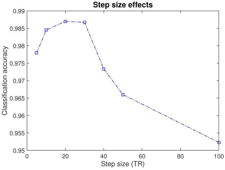
The DCL model was applied to three types of fMRI data to study brain functional connectivity (FC). It needs a large sample size to train deep networks. However, collecting fMRI data of the brain is expensive and therefore the sample sizes of existing brain fMRI cohorts are limited. A possible way to generate more available data is data augmentation, a widely used strategy in deep learning fields, especially when dealing with images. For image classification, data augmentation techniques, e.g., image rotation [18], image reflection [27], scaling [28], are frequently used to generate more images. When it comes to brain FC data, reasonable data augmentation techniques have also been proposed to generate more data. Brain FC reflects the correlation between different brain nodes (ROIs) across a series of time points. The time points can be the entire scan period or a shorter window of the scan. Therefore, data augmentation can be achieved by calculating the correlations across several shorter time slots, which can be obtained by splitting the long time series. A short time window based technique has been applied to MRI data for data augmentation [29]. In our work we used a sliding window approach [30] to generate more samples. There is a trade-off between the authenticity of augmented data and the sample size of the augmented data. Shorter time slots lead to larger sample size but lower authenticity of augmented data. According to the work [31], the window length of 15 to 30 TR seems reasonable for capturing brain functional connectivity (FC) , which has also been used in several other works [32], [33]. Based on the recommendations in the work of [31] and the empirical experiences in [32], [33], and in order to obtain a more authentic augmented data (i.e., a relatively larger window size is preferable), we set the window length to be 30 TR in our work. The step size had a considerable effect on classification results. We have tested the effect of step size on classification accuracy (age classification using resting state and nback task fMRI) and the result was shown in Fig. 3.

Fig. 3:

The Effect of step size on classification accuracy (age classification using resting state and nback task fMRI).

From Fig. 3, the performance (accuracy) increases as step size decreases from 100 TR to 30 TR. This may be due to the increasing sample size of the augmented data, which helps relieve the over-fitting problem in deep network training. However, as step size decreases from 20 TR to 5 TR, the accuracy even drops a bit. This may be due to the increasing overlap between the sliding windows. New augmented sample will become more dependent due to the increasing overlap and the network (on training set) may have more potential to become over-fitted consequently. As the best performance was achieved at “step size = 20 TR”, we used 20 TR as the step size.

D. Experiments design and results

The DCL’s experiments on brain connectivity focused on two tasks: classification (i.e., to classify different age groups or different cognition/WRAT groups using brain connectivity data), and correlation analysis (i.e., to study the correlation between different intrinsic brain functional networks). The classification task verifies the classification power of the DCL model; and the task of correlation analysis verifies the power of the DCL model in terms of detecting correlations. The original 857 subjects were divided into three sets: training set (40%), tuning set (20%), and testing set (40%). Data augmentation was applied to training, tuning, and testing set separately, and each original subject was augmented by 6-10 folds depending on the length of the fMRI scan. The classification of a subject from testing sets is obtained by merging the classification results of his/her augmented subjects, similar to the process of cancer classification in [34]. For instance, if a subject is augmented by 9 folds, then he/she will be classified to the older age group if more than 5 augmented subjects are classified into the older age group.

Mini-batch SGD was used to solve the optimization problem. Hyper-parameters, including momentum, activation function, learning rate, decay rate, batch size, maximum epochs, number of layers, number of nodes in each layer, and the dimensionality of canonical variables, were selected using the tuning set. The final values of hyper-parameters were 0.9 (momentum), ReLu (activation function), 0.01 (learning rate), 1 (decay rate), 32 (batch size), 20 (maximum epochs), 10 (number of layers), 1536 (number of nodes in middle layers), 100 (number of nodes in output layer). Dropout was used to overcome over-fitting and the dropout probability of the middle layers was set to be 0.5. Batch normalization was implemented after each layer to relieve the scale problem resulting from ReLu activation. The experiments were conducted on a computer with an Intel(R) Xeon(R) CPU (E5-2620 v3 @ 2.40 GHz), a 32G RAM, and a NVIDIA Quadro K2200 GPU.

1). Difference of brain FC between different age groups or different WRAT/cognition groups – classification:

We compared the performance of the DCL model to that of other baseline classifiers, including support vector machine (SVM), deep CCA (DCCA) + SVM, logistic regression (Logist), decision tree (DT), random forest (RF), deep neural network (DNN) + SVM, linear collaborative regression (CR) + SVM. For the networks in DNN, DCCA, and DCL, the detailed architectures and key hyper-parameter settings are: 0.9 (momentum), ReLu (activation function), 0.01 (learning rate), 1 (decay rate), 32 (batch size), 20 (maximum epochs), 10 (number of layers), 1536 (number of nodes in middle layers), 100 (number of nodes in output layer). Linear kernel was used for SVM classifier due to its better experimental performance over other kernel options. The number of trees in RF was set to be 100 considering the trade-off of performance and computational cost. Default values were used for other parameter settings for the sake of fair comparison.

As the work endeavors to contribute to the study of brain development during adolescence stage, it is therefore preferable to investigate the FC difference between “before adolescence” and “after adolescence”. Adolescence is an important stage for both physical and psychological development that generally occurs during the period from the beginning of puberty (age 11-12) to legal adulthood (age 18) ¹. The PNC cohort used in the work was collected from subjects aged 8 to 22, among which roughly 20% are in the age range of 8 to 11 years and roughly 20% are in the age range of 18 to 22 years. In this regard and in order to get a balanced data, we selected the top/bottom 20% (in terms of age) as two age groups. WRAT scores partially reflect the development of the brain. In order to have the same subject group size and to facilitate the comparison (e.g., classifying age groups versus classifying WRAT groups), we also selected the top/bottom 20% (in terms of WRAT score) as two WRAT groups. For age groups, the top 20% (in terms of age) subjects were extracted as young adults group while the bottom 20% were extracted as children group. For cognitive ability group, the top 20% (assessed via the WRAT score) of individuals were extracted as a high cognition group (WRAT 114-145) while the bottom 20% were extracted as a low cognition group (WRAT 55-89). All the pre-processing methods, including data augmentation, data standardization, etc, were performed on training set, tuning set, and test set separately.

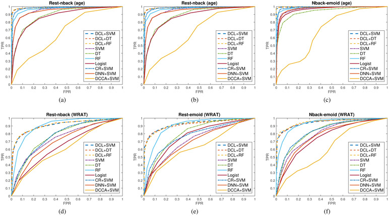
To test the DCL model for multi-modal study, we utilized different data combinations: resting state fMRI and nback task fMRI (rest-nback); resting state fMRI and emoid task fMRI (rest-emoid); nback task fMRI and emoid task fMRI (rest-emoid). For each data combination, we tested the performance of each method, and the results were shown in Fig. 4, Table I, and Table S1-S5. In the experiments, SVM, DT, RF, logistic regression, and DNN concatenated two types of fMRI data as the input, while DCCA, CR, DCL combined two fMRI data using either linear collaborative function or a deep network layer (as shown in Fig. 2). We only included accuracy as a criterion for evaluating classification performance as the two binomial groups had balanced numbers of subjects (top 20% versus bottom 20%). Each experiment was replicated 10 times by re-sampling the training, tuning, and testing sets.

Fig. 4:

The comparison of the ROC curves of different methods in classifying age groups (sub-figs. a-c) and in classifying high/low WRAT groups (sub-figs. d-f). The full names of the methods are deep CCA (DCCA), logistic regression (Logist), support vector machine (SVM), decision tree (DT), random forest (RF), deep neural network (DNN), linear collaborative regression (CR), deep collaborative learning (DCL). In the experiments, SVM, logistic regression, and DNN concatenate two types of fMRI data as the input, while DCCA, CR, DCL combine two fMRI data using either linear collaborative function or a deep network layer. Sub-figs.(a-c) describe the results of classifying age groups using the data combination of rest-nback fMRI, rest-emoid fMRI, and nback-emoid fMRI, respectively. Older age group is defined as positive group. Sub-figs.(d-f) describe the results of classifying WRAT groups using the combination of rest-nback fMRI, rest-emoid fMRI, and nback-emoid fMRI, respectively. Higher WRAT group is defined as positive group.

TABLE I:

The comparison of classification performance (age classification using rest-nback combination). The full names of the measures are: area under ROC curve (AUC), accuracy (ACC), sensitivity (SEN), specificity (SPF), precision (PRC), F1 score (F1).

Classifier	AUC	ACC	SEN	SPF	PRC	F1
DCL+SVM	0.9870	0.9664	0.9500	0.9836	0.9830	0.9660
DCL+DT	0.9872	0.9641	0.9469	0.9823	0.9813	0.9634
DCL+RF	0.9870	0.9672	0.9487	0.9869	0.9860	0.9667
SVM	0.9516	0.8755	0.9145	0.8411	0.8480	0.8784
DT	0.8884	0.8051	0.8604	0.7517	0.7794	0.8162
RF	0.9728	0.9239	0.9079	0.9424	0.9415	0.9224
Logist	0.8747	0.7985	0.8486	0.7499	0.7681	0.8058
CR+SVM	0.9819	0.9445	0.9565	0.9334	0.9329	0.9443
DNN+SVM	0.9456	0.8776	0.9150	0.8448	0.8564	0.8805
DCCA+SVM	0.6703	0.5759	0.5699	0.6033	0.7465	0.5284

From Fig. 4, the proposed model, deep collaborative learning (DCL), achieved better classification performance than other classifiers for both classifying age groups and classifying WRAT groups. Deep CCA obtained the lowest accuracy as it did not capture phenotype related information when doing dimension reduction. Compared with the performances of logistic regression, SVM, and DNN+SVM, both DCL and linear CR achieved better classification performance which demonstrated the correlation information can help get a better representation of the brain connection. DCL’s classification is even more accurate than linear CR due to the incorporation of deep network representation. The high classification accuracy (around 0.95 for age, around 0.80 for WRAT) indicates that both different age groups (e.g., preteens and young adults) and different cognition groups (high WRAT scores and low WRAT scores) may exhibit significantly different brain FC patterns and therefore brain FC may be used as a finger-print to identify different subjects. In addition, it can also be seen from Fig. 4 that the classification accuracy of age groups is higher than that of cognition groups which may be due to the fact that age is a fixed phenotype while cognition score is just a rough measure which is not as accurate and consistent as age.

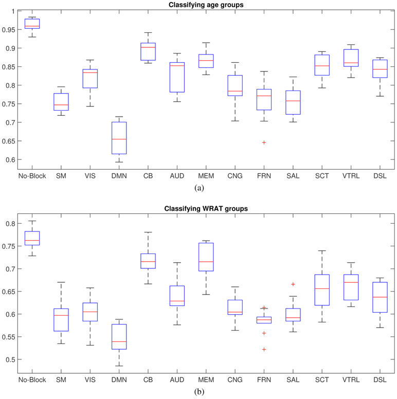
Moreover, as shown in Fig. 4, the combination of two task-fMRI, i.e., nback-emoid, yields much higher classification accuracy than rs-fMRI involved combinations. It indicates that the associations between emotion task fMRI and memory task fMRI were more discriminative and task fMRI may be better for classification or used as finger-print, being consistent with the conclusion in [8]. Furthermore, from Fig. 5, the difference of FCs between young adults and children may be more significant in some networks (e.g., default mode network, sensorimotor network) (because the decreases of accuracy are relatively bigger) and may be relatively less significant in others (e.g. visual network, auditory network, memory network, cerebellum). Similarly, differences in FC between the high and low cognition groups may be more significant in some networks (e.g., default mode network, salience network, sensorimotor network) and may be relatively less significant in others.

Fig. 5:

The classification accuracy in different functional-network-blocked cases. Y-axis represents the classification accuracy. This experiment used the combination of rest fMRI and nback fMRI for classification. In each case, a specific brain subdomain/network was blocked and the rest data were used as the input of the trained network. Sub-fig. (a) describes the result of classifying ages groups; Sub-fig. (b) shows the resulf of classifying WRAT groups. The full names of brain functional networks are sensorimotor network (SM), visual network (VIS), default mode network (DMN), cerebellum (CB), auditory network (AUD), memory retrieval network (MEM), cingulo-opercular task control (CNG), salience network (SAL), subcortical network (SCT), ventral attention (VTRL), dorsal attention (DSL).

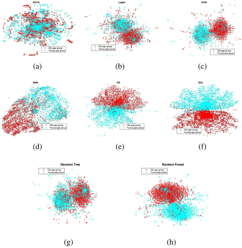
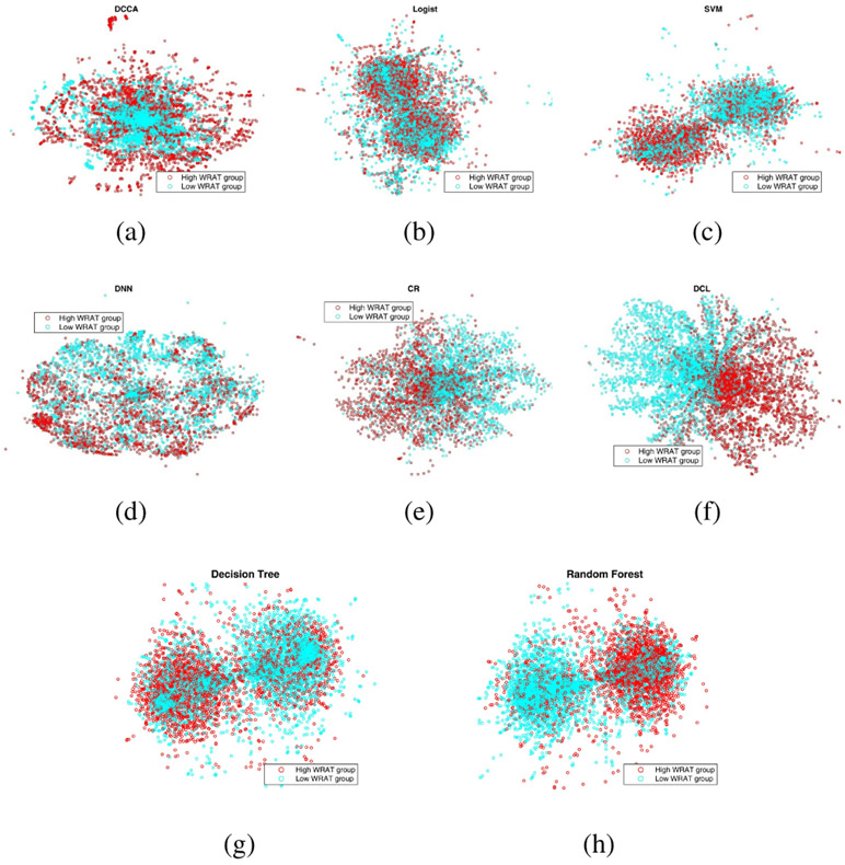
Besides the comparison of accuracy, we visualized the data representations of all the methods. Data visualization was conducted using t-distributed stochastic neighbor embedding (t-SNE) [35], which projects high dimensional data into 2D or 3D spaces for purpose of visualization. The visualization of data representation is shown in Fig. 6 (classifying age groups) and Fig. 7 (classifying WRAT groups). From Fig. 6 and Fig. 7, it is apparent that the representation of DCL has a better discriminative power compared with that of other methods, which also demonstrates the superior performance of the DCL model.

Fig. 6:

The visualization of data representations of different models for classifying age groups. The full names of classifiers can been found in the caption of Fig. 4.

Fig. 7:

The visualization of data representations of different models for classifying WRAT groups. The full names of classifiers can been found in the caption of Fig. 4.

There is great interest in studying how different brain intrinsic functional networks/domains impact the classification accuracy of age groups and WRAT groups, which in return indicates whether different age groups or WRAT groups exhibit different brain connectivity patterns in a specific functional network. However, the data representation of DCL is generated by deep networks in which nonlinear activation functions are applied to each intermediate layer. As a result, it is difficult to interpret how each original feature/variable is represented in the network representation and therefore it is challenging to analyze the discriminative power of each original feature. To partially analyze how different brain intrinsic networks affect the classification accuracy of age groups and WRAT groups, we blocked the signals of each functional network, e.g., DMN, individually and tested how DCL’s classification accuracy changed accordingly. The classification accuracy under each functional-network-block case was shown in Fig. 5. Larger decrease of the accuracy implies that the blocked network/domain is more important for classification and vice versa.

2). Functional connectivity (FC) between different brain networks – correlation analysis:

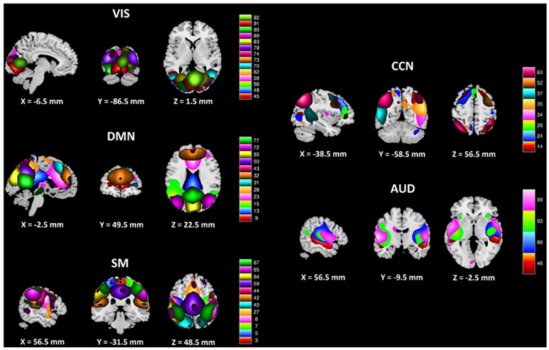
It is also of interest to investigate how brain connectivity between different functional networks changes and how different brain networks cooperate and connect with each other. To study brain FC, both deep collaborative learning (DCL) and linear CCA were applied to the PNC data for correlation analysis after preprocessing resting state fMRI using group independent component analysis (gICA) [36]. The parameter setting and component selection followed those in the work of [30]. A relatively large number of ICA components (100 ICA components) were used to achieve a functional parcellation. Following the critera in Allen et al.’s work [37], we selected a subset of 50 components as intrinsic network components, as opposed to physiological, movement related, or imaging artifacts (ARTs). Dynamic range and low frequency to high frequency ratio were used [30], [37] as the criteria for component selection. The function of each ICA component was then identified based on the Neurosynth database (http://neurosynth.org/) using their coordinates in the Montreal Neurological Institute (MNI) space. The locations of the components of each intrinsic brain network are provided in Fig. 8.

Fig. 8:

A figure showing the sagittal, coronal, and transverse views of brain functional networks extracted by group ICA. The color bar indicates different ICA components. The full names of the brain functional networks are: visual network (VIS), cognitive control network (CCN), auditory network (AUD), default mode network (DMN), and sensorimotor network (SM).

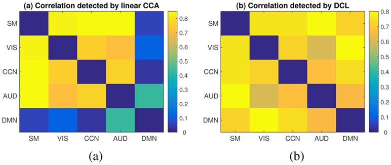
Both linear CCA and DCL were applied to the training set to train the model and then the trained canonical vectors and deep networks were applied to the testing set to calculate test correlations. The test correlations between different brain networks were shown in Fig. 9, in which sub-fig. (a) described correlations detected by linear CCA and sub-fig. (b) described those of DCL. The test correlations shown in Fig. 9 represent multivariate correlations between two functional networks since CCA is a multivariate method. The detected correlations were significant (with significant value < 1e-5) according to Eq. 14.

Fig. 9:

The heatmap showing the correlations (testing set) between different functional networks. (a) describes the results by linear CCA; (b) describes the results by deep collaborative learning (DCL). The color bar indicates the value of detected correlations. The full names of the brain functional networks can be found in the caption of Fig. 8.

As shown in Fig. 9, linear CCA detected strong correlations (above 0.7) between some functional networks, e.g., visual network (VIS), auditory network (AUD), sensorimotor network (SM), and cognitive control network (CCN). However, the correlations between default mode network (DMN) and the rest networks were much weaker (0.43 between DMN and AUD, ~0.1 between DMN and the rest three networks). It is consistent with the the current knowledge about DMN, which exhibits high connectivity within itself but low connections with other networks in the brain [38]. Similar to linear CCA, the DCL model detected strong correlations (above 0.6) between functional networks VIS, AUD, SM, and CCN. However, the DCL model also detected strong correlations between DMN and the rest (VIS, AUD, SM, CCN), which was different from the finding of linear CCA and also different from the current knowledge of DMN network. The different findings between linear CCA and the DCL might indicate that DMN network has some nonlinear correlations and complicated connections with other networks in the brain.

3). Age effects – correlation analysis:

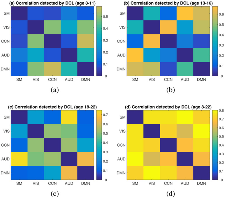
It is of interest to research the effect of age on brain connectivity, which may help better understand the process of brain maturity/development. To investigate the difference of brain connectivity between different age groups, we first selected three age groups: children group (8-11 years), young teenager group (13-16 years), young adult group (18-22 years). Subjects aged 12 and 17 years were excluded in order to get a clear boundary between different age groups. The DCL model was then applied to each age group to analyze the FC between brain networks in resting state. The detected connections between brain subnetworks for each age group were shown in Fig. 10.

Fig. 10:

The heatmap showing age differences in brain connectivity links in resting state. Sub-figs. (a-d) describes the brain FC for age group 8-11 (years), age group 13-16 (years), age group 18-22 (years), and age group 8-22 (years), respectively. The color bar indicates the value of detected correlations. The full names of the brain functional networks can be found in the caption of Fig. 8.

From Fig. 10 (a-c), the patterns of the connections differ between different age groups. For instance, the overall connections between brain sub-networks are relatively weaker at age 8-11 but become relatively stronger at age 13-16 and age 18-22. It demonstrates that the connections of the brain become stronger and stronger during adolescence, as a result of the training and development of the brain with multiple types of brain activities. Moreover, several connections show different pattern at different brain maturity stages (or different age groups). For example, DMN network shows stronger connection with visual network and cognitive network at age 8-11, while its connection with sensorimotor and visual networks become stronger at age 13-16, and it becomes more connected with auditory network at age 18-22. In addition, the connection between cognitive network and visual network is strong throughout the adolescence (age 8-22) while the connection between cognitive network and auditory network becomes strong at a relatively older age stage (18-22).

IV. Discussion and Conclusion

In this work we propose the DCL model to effectively exploit the information from multimodal data using deep networks. DCL seeks the optimal network representation that can maximize cross-data correlation while minimize the data fitting error. As we have demonstrated, the DCL model overcomes the limitations of several existing models (e.g., CCA, deep CCA, collaborative regression) in that it can detect complex/nonlinear cross-data correlations, while extract phenotype related information. In this way, the model can lead to better performance in both prediction and correlation detection. The superior power of DCL on both correlation detection and classification makes it a suitable model for brain FC study, where we apply the model to analyze the correlations of functional networks and the difference of brain connectivity patterns between different subject groups.

As a demonstration, the proposed model, DCL, was applied to the PNC cohort for brain FC study. DCL, as well as other state-of-the-art methods, was used to classify both different age groups and different cognition groups. From the results, DCL performed better than other competitive classifiers, which demonstrated that the incorporation of deep networks into collaborative regression can help achieve higher classification accuracy. Moreover, brain connectivity tends to be more discriminative when used to classify age groups than to classify WRAT/cognition groups. Further experiments showed that the FCs in DMN had more discriminative power while MEM and CB may be less important for classification, which indicated different subject groups exhibited more significant difference in the FC of DMN while relatively less significant difference in MEM and CB. In addition, both DCL and linear CCA were used to investigate how different brain intrinsic networks interacted with each other. In CCA’s results, the correlations between default mode network (DMN) and other networks were weak. In comparison, DCL detected stronger correlations between DMN and other brain networks. The strong nonlinear correlations between DMN and other brain networks might be a new discovery as the connectivity in DMN is normally considered to be distinct from that in other brain networks. Furthermore, brain FCs exhibit different patterns at different maturity stages and the connections of the brain become stronger and stronger during the adolescence stage, according to the analysis of age effects. In summary, DCL outperforms other multimodal fusion models, e.g., deep CCA, linear CR, SVM,and DNN (using concatenated data), for the integration of multiple brain imaging data.

Both age and WRAT score were used in this work by DCL to learn the deep network representation of brain FC. The performance of DCL verified its best network representation of multi-modal data and the trained network can be used for further study by serving as the initial network, similar to the idea of transfer learning. Moreover, DCL could be further improved by employing other network structures, e.g., convolutional neural network (CNN), which can take advantage of the local information of images and reduce computational cost by enforcing shared weights across all nodes. However, directly applying CNN to brain connectivity study may face some difficulties because brain connectivity does not have as strong local information (e.g., shapes) as structural brain images have, needed for CNN models [39]. Despite the challenges of applying CNN based networks, using graph guided network structure [40] may be a promising way to exploit the subtle and complex information within brain connectivity data.

Appendix

The derivation of the gradient of deep collaborative learning

Assume we have two modal data $Z_1\in {\mathbb{R}}^{n\times p}$, $Z_2\in {\mathbb{R}}^{n\times q}$ and a phenotype or label data $Y\in {\mathbb{R}}^{n\times 1}$, where n denotes sample size (number of subjects) and p, q are the dimensionality of feature of Z₁, Z₂ respectively. Then the objective function of deep collaborative learning method is

$$\begin{gathered} (Z_1^{\ast },Z_2^{\ast })=\underset{Z_1,Z_2}{\text{argmax}}\{\underset{U_1,U_2}{\max }\text{Trace}(U_1^{\prime }{Z}_1^{\prime }{Z}_2{U}_2) \\ -\underset{{\beta }_1}{\text{min}}\Vert Y-Z_1{\beta }_1{\Vert }_2^2-\underset{{\beta }_2}{\text{min}}\Vert Y-Z_2{\beta }_2{\Vert }_2^2\} \end{gathered}$$ (15)

$$\begin{gathered} =\underset{Z_1,Z_2}{\text{argmax}}\{\Vert {\Sigma }_{11}^{-\frac{1}{2}}{\Sigma }_{12}{\Sigma }_{22}^{-\frac{1}{2}}\Vert tr \\ -\Vert Y-Z_1(Z_1^{\prime }{Z}_1{)}^{-1}{Z}_1^{\prime }Y{\Vert }_2^2 \\ -\Vert Y-Z_2(Z_2^{\prime }{Z}_2{)}^{-1}{Z}_2^{\prime }Y{\Vert }_2^2\} \end{gathered}$$ (16)

$$=\underset{Z_1,Z_2}{\text{argmax}}F(Z_1,Z_2)$$ (17)

where $Z_1=f_1(X_1)Z_2=f_2(X_2),{\Sigma }_{ij}=Z_i^{\prime }{Z}_j$ f₁, f₂ are two deep networks, $\Vert A{\Vert }_{tr}≔\text{Trace}(\sqrt{A^{\prime }A})=\Sigma {\sigma }_i$ U₁, U₂ in Eq. 15 subject to $U_1^{\prime }{\Sigma }_{11}{U}_1=U_2^{\prime }{\Sigma }_{22}{U}_2=\mathbf{I}$

The gradient of objective function 16 is

$$\begin{gathered} \frac{\partial F(Z_1,Z_2)}{\partial Z_1}=-Z_1{\Sigma }_{11}^{-\frac{1}{2}}UD{U}^{\prime }{\Sigma }_{11}^{-\frac{1}{2}}+Z_2{\Sigma }_{22}^{-\frac{1}{2}}V{U}^{\prime }{\Sigma }_{11}^{-\frac{1}{2}} \\ +2Y{Y}^{\prime }{Z}_1(Z_1^{\prime }{Z}_1{)}^{-1} \\ -2Z_1(Z_1^{\prime }{Z}_1{)}^{-1}{Z}_1^{\prime }Y{Y}^{\prime }{Z}_1(Z_1^{\prime }{Z}_1{)}^{-1} \end{gathered}$$ (18)

$$\begin{gathered} \frac{\partial F(Z_1,Z_2)}{\partial Z_2}=-Z_2{\Sigma }_{22}^{-\frac{1}{2}}VD{V}^{\prime }{\Sigma }_{22}^{-\frac{1}{2}}+Z_1{\Sigma }_{11}^{-\frac{1}{2}}U{V}^{\prime }{\Sigma }_{22}^{-\frac{1}{2}} \\ +2Y{Y}^{\prime }{Z}_2(Z_2^{\prime }{Z}_2{)}^{-1} \\ -2Z_2(Z_2^{\prime }{Z}_2{)}^{-1}{Z}_2^{\prime }Y{Y}^{\prime }{Z}_2(Z_2^{\prime }{Z}_2{)}^{-1} \end{gathered}$$ (19)

where $[U,D,V]=\text{svd}({\Sigma }_{11}^{-\frac{1}{2}}{\Sigma }_{12}{\Sigma }_{22}^{-\frac{1}{2}})$

We will prove Eq. 18 in the following sections, and Eq. 19 is straightforward to get because it is a symmetric expression of Eq. 18. Let $T_1=Z_1(Z_1^{\prime }{Z}_1{)}^{-1}{Z}_1^{\prime }$, $T_2=Z_2(Z_2^{\prime }{Z}_2{)}^{-1}{Z}_2^{\prime }$. To prove Eq. 18, we just need to prove

$$\begin{gathered} \frac{\partial \Vert Y-T_{1}Y{\Vert }_2^2}{\partial Z_1}=2Y{Y}^{\prime }{Z}_1(Z_1^{\prime }{Z}_1{)}^{-1} \\ -2Z_1(Z_1^{\prime }{Z}_1{)}^{-1}{Z}_1^{\prime }Y{Y}^{\prime }{Z}_1(Z_1^{\prime }{Z}_1{)}^{-1} \end{gathered}$$ (20)

$$\begin{gathered} \frac{\partial }{\partial Z_1}\Vert {\Sigma }_{11}^{-\frac{1}{2}}{\Sigma }_{12}{\Sigma }_{22}^{-\frac{1}{2}}{\Vert }_{tr}=-Z_1{\Sigma }_{11}^{-\frac{1}{2}}UD{U}^{\prime }{\Sigma }_{11}^{-\frac{1}{2}} \\ +Z_2{\Sigma }_{22}^{-\frac{1}{2}}V{U}^{\prime }{\Sigma }_{11}^{-\frac{1}{2}} \end{gathered}$$ (21)

To prove Eq. 20, we have

$$\frac{\partial \Vert Y-T_{1}Y{\Vert }_2^2}{\partial Z_1}=\frac{\partial }{\partial Z_1}\{Y^{\prime }{T}_1^{\prime }{T}_{1}Y-Y^{\prime }{T}_1^{\prime }Y-Y^{\prime }{T}_{1}Y+Y^{\prime }Y\}$$ (22)

$$\begin{gathered} =\frac{\partial }{\partial Z_1}\{Y^{\prime }{T}_1{T}_{1}Y-2Y^{\prime }{T}_{1}Y\} \\ (\text{because}{T}_1^{\prime }=T_1) \end{gathered}$$ (23)

Inserting $T_1=Z_1(Z_1^{\prime }{Z}_1{)}^{-1}{Z}_1^{\prime }$ into Y′T₁T₁Y gives

$$\begin{gathered} Y^{\prime }{T}_1{T}_{1}Y=Y^{\prime }{Z}_1(Z_1^{\prime }{Z}_1{)}^{-1}{Z}_1^{\prime }{Z}_1(Z_1^{\prime }{Z}_1{)}^{-1}{Z}_1^{\prime }Y \\ =Y^{\prime }{Z}_1(Z_1^{\prime }{Z}_1{)}^{-1}{Z}_1^{\prime }Y \\ =Y^{\prime }{T}_{1}Y \end{gathered}$$ (24)

From Eqs. 23 and 24, we have

$$\begin{gathered} \frac{\partial \Vert Y-T_{1}Y{\Vert }_2^2}{\partial Z_1}=-\frac{\partial }{\partial Z_1}\{Y^{\prime }{T}_{1}Y\} \\ =\frac{\partial }{\partial Z_1}{Y}^{\prime }{Z}_1(Z_1^{\prime }{Z}_1{)}^{-1}{Z}_1^{\prime }Y \\ =\frac{\partial }{\partial Z_1}{Y}^{\prime }{Z}_1^c(Z_1^{c\prime }{Z}_1^c{)}^{-1}{Z}_1^{\prime }Y+\frac{\partial }{\partial Z_1}{Y}^{\prime }{Z}_1(Z_1^{c\prime }{Z}_1^c{)}^{-1}{Z}_1^{c\prime }Y+ \end{gathered}$$ (25)

$$\begin{gathered} \frac{\partial }{\partial Z_1}{Y}^{\prime }{Z}_1^c(Z_1^{c\prime }{Z}_1{)}^{-1}{Z}_1^{c\prime }Y+\frac{\partial }{\partial Z_1}{Y}^{\prime }{Z}_1^c(Z_1^{\prime }{Z}_1^c{)}^{-1}{Z}_1^{c\prime }Y \\ =2(\frac{\partial }{\partial Z_1}{Y}^{\prime }{Z}_1(Z_1^{c\prime }{Z}_1^c{)}^{-1}{Z}_1^{c\prime }Y+\frac{\partial }{\partial Z_1}{Y}^{\prime }{Z}_1^c(Z_1^{\prime }{Z}_1^c{)}^{-1}{Z}_1^{c\prime }Y) \end{gathered}$$ (26)

Note that in Eqs. 25-26 we treat some Z₁ as constant by replacing Z₁ with $Z_1^c$, and therefore $Z_1^c$ satisfies $\frac{\partial Z_1^c}{\partial Z_1}=0$. To prove Eq. 20, from Eqs. 26 and 20, we just need to prove

$$\frac{\partial }{\partial Z_1}{Y}^{\prime }{Z}_1(Z_1^{c\prime }{Z}_1^c{)}^{-1}{Z}_1^{c\prime }Y=Y{Y}^{\prime }{Z}_1(Z_1^{\prime }{Z}_1{)}^{-1}$$ (27)

and

$$\begin{gathered} \frac{\partial }{\partial Z_1}{Y}^{\prime }{Z}_1^c(Z_1^{\prime }{Z}_1^c{)}^{-1}{Z}_1^{c\prime }Y= \\ -Z_1(Z_1^{\prime }{Z}_1{)}^{-1}{Z}_1^{\prime }Y{Y}^{\prime }{Z}_1(Z_1^{\prime }{Z}_1{)}^{-1} \end{gathered}$$ (28)

For the purpose of convenience, we replace Z₁ with Z in the following sections. As a result, Eqs. 27 and 28 become

$$\frac{\partial }{\partial Z}{Y}^{\prime }Z(Z^{c\prime }{Z}^c{)}^{-1}{Z}^{c\prime }Y=Y{Y}^{\prime }Z(Z^{\prime }Z{)}^{-1}$$ (29)

and

$$\frac{\partial }{\partial Z}{Y}^{\prime }{Z}^c(Z^{\prime }{Z}^c{)}^{-1}{Z}^{c\prime }Y=-Z(Z^{\prime }Z{)}^{-1}{Z}^{\prime }Y{Y}^{\prime }Z(Z^{\prime }Z{)}^{-1}$$ (30)

To prove Eq. 29

$$\frac{\partial }{\partial Z}{Y}^{\prime }Z(Z^{c\prime }{Z}^c{)}^{-1}{Z}^{c\prime }Y$$ (31)

$$\begin{gathered} =\frac{\partial }{\partial Z}\text{Trace}(Y^{\prime }Z(Z^{c\prime }{Z}^c{)}^{-1}{Z}^{c\prime }Y) \\ =\frac{\partial }{\partial Z}\text{Trace}(Z(Z^{c\prime }{Z}^c{)}^{-1}{Z}^{c\prime }Y{Y}^{\prime }) \end{gathered}$$ (32)

From $\frac{\partial }{\partial X}\text{Trace}(XA)=A^{\prime }$ (Eq. (100) in [41]),

$$32=((Z^{c\prime }{Z}^c{)}^{-1}{Z}^{c\prime }Y{Y}^{\prime }{)}^{\prime }$$ (33)

$$=Y{Y}^{\prime }Z(Z^{\prime }Z{)}^{-1}$$ (34)

To prove Eq. 30, following the chain rule of matrix derivative $\frac{\partial g(U)}{\partial X}=\frac{\partial g(U)}{\partial x_{ij}}={\sum }_{k,l}\frac{\partial g(U)}{\partial u_{kl}}=\frac{\partial u_{kl}}{\partial x_{ij}}$ (Eq. (136) in [41])

$$\begin{gathered} \frac{\partial }{\partial Z}{Y}^{\prime }{Z}^c(Z^{\prime }{Z}^c{)}^{-1}{Z}^{c\prime }Y \\ =\frac{\partial }{\partial Z}\text{Trace}(Y^{\prime }{Z}^c(Z^{\prime }{Z}^c{)}^{-1}{Z}^{c\prime }Y) \\ =\frac{\partial }{\partial z_{ij}}\text{Trace}((Z^{\prime }{Z}^c{)}^{-1}{Z}^{c\prime }Y{Y}^{\prime }{Z}^c) \\ =\sum _{k,l}\frac{\partial }{\partial (Z^{\prime }{Z}^c{)}_{kl}}\text{Trace}((Z^{\prime }{Z}^c{)}^{-1}{Z}^{c\prime }Y{Y}^{\prime }{Z}^c\frac{\partial (Z^{\prime }{Z}^c{)}_{kl}}{\partial z_{ij}} \end{gathered}$$ (35)

From $\frac{\partial \text{Trace}(A{X}^{-1}B)}{\partial X}=-(X^{-1}BA{X}^{-1}{)}^{\prime }$ (Eq. (63) in [41]) and $\frac{\partial {\left(X^{\prime }A\right)}_{ij}}{\partial X_{mn}}={\left(J^{nm}A\right)}_{ij}$, where J^nm is the single-entry matrix, 1 at (n, m) and 0 elsewhere (Eq. (75) in [41]), we have

$$\begin{gathered} 35=\sum _{k,l}\{-((Z^{\prime }{Z}^c{)}^{-1}{Z}^{c\prime }Y{Y}^{\prime }{Z}^c(Z^{\prime }{Z}^c{)}^{-1}{)}^{\prime }{\}}_{kl}\frac{\partial (Z^{\prime }{Z}^c{)}_{kl}}{\partial z_{ij}} \\ =\sum _{k,l}\{-(Z^{\prime }Z{)}^{-1}{Z}^{\prime }Y{Y}^{\prime }Z(Z^{\prime }Z{)}^{-1}{\}}_{kl}(J^{ji}Z{)}_{kl} \\ =\sum _l\{-((Z^{\prime }Z{)}^{-1}{Z}^{\prime }Y{Y}^{\prime }Z(Z^{\prime }Z{)}^{-1}{\}}_{jl}{Z}_{il} \\ =\sum _l{Z}_{il}\{-(Z^{\prime }Z{)}^{-1}{Z}^{\prime }Y{Y}^{\prime }Z(Z^{\prime }Z{)}^{-1}{\}}_{lj} \\ =-Z(Z^{\prime }Z{)}^{-1}{Z}^{\prime }Y{Y}^{\prime }Z(Z^{\prime }Z{)}^{-1} \end{gathered}$$ (36)

Thus Eq. 20 is proved.

To prove Eq. 21, we just need to calculate $\frac{\partial }{\partial {\Sigma }_{11}}\Vert {\Sigma }_{11}^{-\frac{1}{2}}{\Sigma }_{12}{\Sigma }_{22}^{-\frac{1}{2}}{\Vert }_{tr}$ and $\frac{\partial }{\partial {\Sigma }_{12}}\Vert {\Sigma }_{11}^{-\frac{1}{2}}{\Sigma }_{12}{\Sigma }_{22}^{-\frac{1}{2}}{\Vert }_{tr}$ so that Eq. 21 can be calculated using the chain rule (the rest of the proof is similar to that in [17]). From [42], we have

$$\forall \text{matrix}A,\frac{\partial }{\partial A}\Vert A{\Vert }_{tr}=U{V}^{\prime },$$ (37)

where [U, D, V] = svd(A), and the trace norm is defined as $\Vert A{\Vert }_{tr}≔\text{Trace}(\sqrt{A^{\prime }A})$.

Using Eq. 37 and the chain rule

$$\begin{gathered} \frac{\partial }{\partial {\left({\Sigma }_{12}\right)}_{ij}}\Vert {\Sigma }_{11}^{-\frac{1}{2}}{\Sigma }_{12}{\Sigma }_{22}^{-\frac{1}{2}}{\Vert }_{tr} \\ =\sum _{k,l}\frac{\partial \Vert {\Sigma }_{11}^{-\frac{1}{2}}{\Sigma }_{12}{\Sigma }_{22}^{-\frac{1}{2}}{\Vert }_{tr}}{\partial ({\Sigma }_{11}^{-\frac{1}{2}}{\Sigma }_{12}{\Sigma }_{22}^{-\frac{1}{2}}{)}_{kl}}\cdot \frac{\partial ({\Sigma }_{11}^{-\frac{1}{2}}{\Sigma }_{12}{\Sigma }_{22}^{-\frac{1}{2}}{)}_{kl}}{\partial {\left({\Sigma }_{12}\right)}_{ij}} \\ =\sum _{k,l}(U{V}^{\prime }{)}_{kl}({\Sigma }_{11}^{-\frac{1}{2}}{)}_{ki}({\Sigma }_{22}^{-\frac{1}{2}}{)}_{jl} \\ =\sum _{k,l}({\Sigma }_{11}^{-\frac{1}{2}}{)}_{ik}(U{V}^{\prime }{)}_{kl}({\Sigma }_{22}^{-\frac{1}{2}}{)}_{lj} \end{gathered}$$ (38)

$$=({\Sigma }_{11}^{-\frac{1}{2}}U{V}^{\prime }{\Sigma }_{22}^{-\frac{1}{2}}{)}_{ij}$$ (39)

where $[U,D,V]=\text{svd}({\Sigma }_{11}^{-\frac{1}{2}}{\Sigma }_{12}{\Sigma }_{22}^{-\frac{1}{2}})$.

From [17], we have

$$\frac{\partial \text{Trace}(X^{\frac{1}{2}})}{\partial X}=\frac{1}{2}{X}^{-\frac{1}{2}}$$ (40)

Using Eq. 40 and the chain rule

$$\begin{gathered} \frac{\partial }{\partial {\left({\Sigma }_{11}\right)}_{ij}}\Vert {\Sigma }_{11}^{-\frac{1}{2}}{\Sigma }_{12}{\Sigma }_{22}^{-\frac{1}{2}}{\Vert }_{tr} \\ =\frac{\partial }{\partial {\left({\Sigma }_{11}\right)}_{ij}}\text{Trace}\{({\Sigma }_{22}^{-\frac{1}{2}}{\Sigma }_{21}{\Sigma }_{11}^{-1}{\Sigma }_{12}{\Sigma }_{22}^{-\frac{1}{2}}{)}^{-\frac{1}{2}}\} \\ =\sum _{k,l}\frac{\partial \text{Trace}\{({\Sigma }_{22}^{-\frac{1}{2}}{\Sigma }_{21}{\Sigma }_{11}^{-1}{\Sigma }_{12}{\Sigma }_{22}^{-\frac{1}{2}}{)}^{\frac{1}{2}}\}}{\partial ({\Sigma }_{22}^{-\frac{1}{2}}{\Sigma }_{21}{\Sigma }_{11}^{-1}{\Sigma }_{12}{\Sigma }_{22}^{-\frac{1}{2}}{)}_{kl}} \\ \cdot \frac{\partial ({\Sigma }_{22}^{-\frac{1}{2}}{\Sigma }_{21}{\Sigma }_{11}^{-1}{\Sigma }_{12}{\Sigma }_{22}^{-\frac{1}{2}}{)}_{kl}}{\partial ({\Sigma }_{11}{)}_{ij}} \end{gathered}$$ (41)

$$\begin{gathered} =\sum _{k,l}(\frac{1}{2}({\Sigma }_{22}^{-\frac{1}{2}}{\Sigma }_{21}{\Sigma }_{11}^{-1}{\Sigma }_{12}{\Sigma }_{22}^{-\frac{1}{2}}{)}^{-\frac{1}{2}}{)}_{kl} \\ \cdot \frac{\partial ({\Sigma }_{22}^{-\frac{1}{2}}{\Sigma }_{21}{\Sigma }_{11}^{-1}{\Sigma }_{12}{\Sigma }_{22}^{-\frac{1}{2}}{)}_{kl}}{\partial ({\Sigma }_{11}{)}_{ij}} \end{gathered}$$ (42)

Before deriving the final expression of Eq. 42, we calculate $\frac{\partial {\left({\Sigma }_{22}^{-\frac{1}{2}}{\Sigma }_{21}{\Sigma }_{11}^{-1}{\Sigma }_{12}{\Sigma }_{22}^{-\frac{1}{2}}\right)}_{kl}}{\partial {\left({\Sigma }_{11}\right)}_{ij}}$ using $\frac{\partial (X^{-1}{)}_{kl}}{\partial X_{ij}}=-(X^{-1}{)}_{ki}(X^{-1}{)}_{jl}$ (Eq. (60) in [41]) and the chain rule,

$$\begin{gathered} \frac{\partial {\left({\Sigma }_{22}^{-\frac{1}{2}}{\Sigma }_{21}{\Sigma }_{11}^{-1}{\Sigma }_{12}{\Sigma }_{22}^{-\frac{1}{2}}\right)}_{kl}}{\partial {\left({\Sigma }_{11}\right)}_{ij}} \\ =\sum _{a,b}\frac{{\left({\Sigma }_{22}^{-\frac{1}{2}}{\Sigma }_{21}{\Sigma }_{11}^{-1}{\Sigma }_{12}{\Sigma }_{22}^{-\frac{1}{2}}\right)}_{kl}}{\partial {\left({\Sigma }_{11}^{-1}\right)}_{ab}}\cdot \frac{\partial {\left({\Sigma }_{11}^{-1}\right)}_{ab}}{\partial {\left({\Sigma }_{11}\right)}_{ij}} \\ =-\sum _{a,b}({\Sigma }_{22}^{-\frac{1}{2}}{\Sigma }_{21}{)}_{ka}({\Sigma }_{12}{\Sigma }_{22}^{-\frac{1}{2}}{)}_{bl}({\Sigma }_{11}^{-1}{)}_{ai}({\Sigma }_{11}^{-1}{)}_{jb} \\ =-\sum _{a,b}({\Sigma }_{22}^{-\frac{1}{2}}{\Sigma }_{21}{)}_{ka}({\Sigma }_{11}^{-1}{)}_{ai}({\Sigma }_{11}^{-1}{)}_{jb}({\Sigma }_{12}{\Sigma }_{22}^{-\frac{1}{2}}{)}_{bl} \end{gathered}$$ (43)

$$=-({\Sigma }_{22}^{-\frac{1}{2}}{\Sigma }_{21}{\Sigma }_{11}^{-1}{)}_{ki}({\Sigma }_{11}^{-1}{\Sigma }_{12}{\Sigma }_{22}^{-\frac{1}{2}}{)}_{jl}$$ (44)

Now we can derive Eq. 42 with the help of Eq. 44,

$$\begin{gathered} \frac{\partial }{\partial {\left({\Sigma }_{11}\right)}_{ij}}\Vert {\Sigma }_{11}^{-\frac{1}{2}}{\Sigma }_{12}{\Sigma }_{22}^{-\frac{1}{2}}{\Vert }_{tr} \\ =42-\sum _{k,l}(\frac{1}{2}({\Sigma }_{22}^{-\frac{1}{2}}{\Sigma }_{21}{\Sigma }_{11}^{-1}{\Sigma }_{12}{\Sigma }_{22}^{-\frac{1}{2}}{)}^{-\frac{1}{2}}{)}_{kl} \\ \cdot ({\Sigma }_{22}^{-\frac{1}{2}}{\Sigma }_{21}{\Sigma }_{11}^{-1}{)}_{ki}({\Sigma }_{11}^{-1}{\Sigma }_{12}{\Sigma }_{22}^{-\frac{1}{2}}{)}_{jl} \\ =-\frac{1}{2}\sum _{k,l}({\Sigma }_{11}^{-1}{\Sigma }_{12}{\Sigma }_{22}^{-\frac{1}{2}}{)}_{ik} \\ \cdot (({\Sigma }_{22}^{-\frac{1}{2}}{\Sigma }_{21}{\Sigma }_{11}^{-1}{\Sigma }_{12}{\Sigma }_{22}^{-\frac{1}{2}}{)}^{-\frac{1}{2}}{)}_{kl}({\Sigma }_{22}^{-\frac{1}{2}}{\Sigma }_{21}{\Sigma }_{11}^{-1}{)}_{lj} \\ =-\frac{1}{2}\{{\Sigma }_{11}^{-1}{\Sigma }_{12}{\Sigma }_{22}^{-\frac{1}{2}}({\Sigma }_{22}^{-\frac{1}{2}}{\Sigma }_{21}{\Sigma }_{11}^{-1}{\Sigma }_{12}{\Sigma }_{22}^{-\frac{1}{2}}{)}^{-\frac{1}{2}} \\ \cdot {\Sigma }_{22}^{-\frac{1}{2}}{\Sigma }_{21}{\Sigma }_{11}^{-1}{\}}_{ij} \\ =-\frac{1}{2}\{{\Sigma }_{11}^{-\frac{1}{2}}UD{V}^{\prime }(V{D}^{-1}{V}^{\prime })VD{U}^{\prime }{\Sigma }_{11}^{-\frac{1}{2}}{\}}_{ij} \end{gathered}$$ (45)

$$=-\frac{1}{2}({\Sigma }_{11}^{-\frac{1}{2}}UD{U}^{\prime }{\Sigma }_{11}^{-\frac{1}{2}}{)}_{ij}$$ (46)

With Eqs. 39, 46, now we can calculate Eq. 21

$$\begin{gathered} \frac{\partial }{\partial {\left(Z_1\right)}_{kl}}\Vert {\Sigma }_{11}^{-\frac{1}{2}}{\Sigma }_{12}{\Sigma }_{22}^{-\frac{1}{2}}{\Vert }_{tr} \\ =\sum _{i,j}\frac{\partial \Vert {\Sigma }_{11}^{-\frac{1}{2}}{\Sigma }_{12}{\Sigma }_{22}^{-\frac{1}{2}}{\Vert }_{tr}}{\partial {\left({\Sigma }_{11}\right)}_{ij}}\cdot \frac{\partial {\left({\Sigma }_{11}\right)}_{ij}}{\partial {\left(Z_1\right)}_{kl}} \end{gathered}$$ (47)

$$+\frac{\partial \Vert {\Sigma }_{11}^{-\frac{1}{2}}{\Sigma }_{12}{\Sigma }_{22}^{-\frac{1}{2}}{\Vert }_{tr}}{\partial {\left({\Sigma }_{12}\right)}_{ij}}\cdot \frac{\partial {\left({\Sigma }_{12}\right)}_{ij}}{\partial {\left(Z_1\right)}_{kl}}$$ (48)

From Eq. 46 and $\frac{\partial {\left(X^{\prime }A\right)}_{ij}}{\partial X_{mn}}={\left(J^{nm}A\right)}_{ij}$, where J^nm is the single-entry matrix, 1 at (n, m) and 0 elsewhere (Eq. (75) in [41]), the first term in Eq. 48 can be derived as

$$\begin{gathered} \sum _{i,j}\frac{\partial \Vert {\Sigma }_{11}^{-\frac{1}{2}}{\Sigma }_{12}{\Sigma }_{22}^{-\frac{1}{2}}{\Vert }_{tr}}{\partial {\left({\Sigma }_{11}\right)}_{ij}}\cdot \frac{\partial {\left({\Sigma }_{11}\right)}_{ij}}{\partial {\left(Z_1\right)}_{kl}} \\ =\sum _{i,j}-\frac{1}{2}\{{\Sigma }_{11}^{-\frac{1}{2}}UD{U}^{\prime }{\Sigma }_{11}^{-\frac{1}{2}}{\}}_{ij}\cdot \frac{\partial {\left(Z_1^{\prime }{Z}_1\right)}_{ij}}{\partial {\left(Z_1\right)}_{kl}} \\ =\sum _{i,j}-\frac{1}{2}\{{\Sigma }_{11}^{-\frac{1}{2}}UD{U}^{\prime }{\Sigma }_{11}^{-\frac{1}{2}}{\}}_{ij}\cdot \left((J^{lk}{Z}_1{)}_{ij}+(J^{lk}{Z}_1{)}_{ji}\right) \\ =\sum _j-\frac{1}{2}\{{\Sigma }_{11}^{-\frac{1}{2}}UD{U}^{\prime }{\Sigma }_{11}^{-\frac{1}{2}}{\}}_{lj}\cdot (Z_1{)}_{kj} \\ +\sum _i-\frac{1}{2}\{{\Sigma }_{11}^{-\frac{1}{2}}UD{U}^{\prime }{\Sigma }_{11}^{-\frac{1}{2}}{\}}_{il}\cdot (Z_1{)}_{ki} \\ =\sum _j-\frac{1}{2}(Z_1{)}_{kj}\cdot \{{\Sigma }_{11}^{-\frac{1}{2}}UD{U}^{\prime }{\Sigma }_{11}^{-\frac{1}{2}}{\}}_{jl} \\ +\sum _i-\frac{1}{2}(Z_1{)}_{ki}\cdot \{{\Sigma }_{11}^{-\frac{1}{2}}UD{U}^{\prime }{\Sigma }_{11}^{-\frac{1}{2}}{\}}_{il} \\ =-\frac{1}{2}\{Z_1{\Sigma }_{11}^{-\frac{1}{2}}UD{U}^{\prime }{\Sigma }_{11}^{-\frac{1}{2}}{\}}_{kl}-\frac{1}{2}\{Z_1{\Sigma }_{11}^{-\frac{1}{2}}UD{U}^{\prime }{\Sigma }_{11}^{-\frac{1}{2}}{\}}_{kl} \end{gathered}$$ (49)

$$=-(Z_1{\Sigma }_{11}^{-\frac{1}{2}}UD{U}^{\prime }{\Sigma }_{11}^{-\frac{1}{2}}{)}_{kl}$$ (50)

From Eq. 39 and $\frac{\partial {\left(X^{\prime }A\right)}_{ij}}{\partial X_{mn}}={\left(J^{nm}A\right)}_{ij}$, where J^nm is the single-entry matrix, 1 at (n, m) and 0 elsewhere (Eq. (75) in [41]), the second term in Eq. 48 can be derived as

$$\begin{gathered} \sum _{i,j}\frac{\partial \Vert {\Sigma }_{11}^{-\frac{1}{2}}{\Sigma }_{12}{\Sigma }_{22}^{-\frac{1}{2}}{\Vert }_{tr}}{\partial {\left({\Sigma }_{12}\right)}_{ij}}\cdot \frac{\partial {\left({\Sigma }_{12}\right)}_{ij}}{\partial {\left(Z_1\right)}_{kl}} \\ =\sum _{i,j}({\Sigma }_{11}^{-\frac{1}{2}}U{V}^{\prime }{\Sigma }_{22}^{-\frac{1}{2}}{)}_{ij}\cdot \frac{\partial {\left(Z_1^{\prime }{Z}_2\right)}_{ij}}{\partial {\left(Z_1\right)}_{kl}} \\ =\sum _{i,j}({\Sigma }_{11}^{-\frac{1}{2}}U{V}^{\prime }{\Sigma }_{22}^{-\frac{1}{2}}{)}_{ij}\cdot {\left(J^{lk}{Z}_2\right)}_{ij} \\ =\sum _j({\Sigma }_{11}^{-\frac{1}{2}}U{V}^{\prime }{\Sigma }_{22}^{-\frac{1}{2}}{)}_{lj}\cdot (Z_2{)}_{kj} \\ =\sum _j(Z_2{)}_{kj}\cdot ({\Sigma }_{22}^{-\frac{1}{2}}V{U}^{\prime }{\Sigma }_{11}^{-\frac{1}{2}}{)}_{jl} \end{gathered}$$ (51)

$$=(Z_2{\Sigma }_{22}^{-\frac{1}{2}}V{U}^{\prime }{\Sigma }_{11}^{-\frac{1}{2}}{)}_{kl}$$ (52)

From Eqs. 48, 50, and 52, we have

$$\frac{\partial }{\partial (Z_1{)}_{kl}}\Vert {\Sigma }_{11}^{-\frac{1}{2}}{\Sigma }_{12}{\Sigma }_{22}^{-\frac{1}{2}}{\Vert }_{tr}$$ (53)

= Eq. 48 = Eq. 50 + Eq. 52

$$=-(Z_1{\Sigma }_{11}^{-\frac{1}{2}}UD{U}^{\prime }{\Sigma }_{11}^{-\frac{1}{2}}{)}_{kl}+(Z_2{\Sigma }_{22}^{-\frac{1}{2}}V{U}^{\prime }{\Sigma }_{11}^{-\frac{1}{2}}{)}_{kl}$$ (54)

Thus Eq. 21 is proved.

References

- [1].Calhoun VD and Adali T, “Time-varying brain connectivity in fmri data: whole-brain data-driven approaches for capturing and characterizing dynamic states,” IEEE Signal Processing Magazine, vol. 33, no. 3, pp. 52–66, 2016. [Google Scholar]
- [2].Rubinov M and Sporns O, “Complex network measures of brain connectivity: uses and interpretations,” Neuroimage, vol. 52, no. 3, pp. 1059–1069, 2010. [DOI] [PubMed] [Google Scholar]
- [3].Calhoun VD, Miller R, Pearlson G, and Adalı T, “The chronnectome: time-varying connectivity networks as the next frontier in fmri data discovery,” Neuron, vol. 84, no. 2, pp. 262–274, 2014. [DOI] [PMC free article] [PubMed] [Google Scholar]
- [4].Cai B, Zille P, Stephen JM, Wilson TW, Calhoun VD, and Wang YP, “Estimation of dynamic sparse connectivity patterns from resting state fmri,” IEEE transactions on medical imaging, vol. 37, no. 5, pp. 1224–1234, 2018. [DOI] [PMC free article] [PubMed] [Google Scholar]
- [5].Jolles DD, van Buchem MA, Crone EA, and Rombouts SA, “A comprehensive study of whole-brain functional connectivity in children and young adults,” Cerebral cortex, vol. 21, no. 2, pp. 385–391, 2010. [DOI] [PubMed] [Google Scholar]
- [6].Fair DA, Cohen AL, Power JD, Dosenbach NU, Church JA, Miezin FM, Schlaggar BL, and Petersen SE, “Functional brain networks develop from a local to distributed organization,” PLoS computational biology, vol. 5, no. 5, p. e1000381, 2009. [DOI] [PMC free article] [PubMed] [Google Scholar]
- [7].Zille P, Calhoun VD, Stephen JM, Wilson TW, and Wang Y-P, “Fused estimation of sparse connectivity patterns from rest fmri. application to comparison of children and adult brains,” IEEE transactions on medical imaging, vol. 37, no. 10, pp. 2165–2175, 2018. [DOI] [PMC free article] [PubMed] [Google Scholar]
- [8].Greene AS, Gao S, Scheinost D, and Constable RT, “Task-induced brain state manipulation improves prediction of individual traits,” Nature communications, vol. 9, no. 1, p. 2807, 2018. [DOI] [PMC free article] [PubMed] [Google Scholar]
- [9].Chen S and Hu X, “Individual identification using the functional brain fingerprint detected by the recurrent neural network,” Brain connectivity, vol. 8, no. 4, pp. 197–204, 2018. [DOI] [PubMed] [Google Scholar]
- [10].Plis SM, Amin MF, Chekroud A, Hjelm D, Damaraju E, Lee HJ, Bustillo JR, Cho K, Pearlson GD, and Calhoun VD, “Reading the (functional) writing on the (structural) wall: Multimodal fusion of brain structure and function via a deep neural network based translation approach reveals novel impairments in schizophrenia,” NeuroImage, vol. 181, pp. 734–747, 2018. [DOI] [PMC free article] [PubMed] [Google Scholar]
- [11].Sui J, Pearlson G, Caprihan A, Adali T, Kiehl KA, Liu J, Yamamoto J, and Calhoun VD, “Discriminating schizophrenia and bipolar disorder by fusing fmri and dti in a multimodal cca+ joint ica model,” Neuroimage, vol. 57, no. 3, pp. 839–855, 2011. [DOI] [PMC free article] [PubMed] [Google Scholar]
- [12].Liu J, Demirci O, and Calhoun VD, “A parallel independent component analysis approach to investigate genomic influence on brain function,” IEEE signal processing letters, vol. 15, p. 413, 2008. [DOI] [PMC free article] [PubMed] [Google Scholar]
- [13].Ngiam J, Khosla A, Kim M, Nam J, Lee H, and Ng AY, “Multimodal deep learning,” in Proceedings of the 28th international conference on machine learning (ICML-11), pp. 689–696, 2011. [Google Scholar]
- [14].Gross SM and Tibshirani R, “Collaborative regression,” Biostatistics, vol. 16, no. 2, pp. 326–338, 2014. [DOI] [PMC free article] [PubMed] [Google Scholar]
- [15].Hotelling H, “Relations between two sets of variates,” Biometrika, vol. 28, pp. 321–377, 1936. [Google Scholar]
- [16].Tibshirani R, “Regression shrinkage and selection via the lasso,” Journal of the Royal Statistical Society. Series B (Methodological), pp. 267–288, 1996. [Google Scholar]
- [17].Andrew G, Arora R, Bilmes J, and Livescu K, “Deep canonical correlation analysis,” in International Conference on Machine Learning, pp. 1247–1255, 2013. [Google Scholar]
- [18].Wang W, Arora R, Livescu K, and Bilmes J, “On deep multi-view representation learning,” in International Conference on Machine Learning, pp. 1083–1092, 2015. [Google Scholar]
- [19].Marcoulides GA and Hershberger SL, Multivariate statistical methods: A first course. Psychology Press, 2014. [Google Scholar]
- [20].Bartlett M, “The statistical significance of canonical correlations,” Biometrika, vol. 32, no. 1, pp. 29–37, 1941. [Google Scholar]
- [21].Satterthwaite TD, Elliott MA, Ruparel K, Loughead J, Prabhakaran K, Calkins ME, Hopson R, Jackson C, Keefe J, Riley M, et al. , “Neuroimaging of the philadelphia neurodevelopmental cohort,” Neuroimage, vol. 86, pp. 544–553, 2014. [DOI] [PMC free article] [PubMed] [Google Scholar]
- [22].Ragland JD, Turetsky BI, Gur RC, Gunning-Dixon F, Turner T, Schroeder L, Chan R, and Gur RE, “Working memory for complex figures: an fmri comparison of letter and fractal n-back tasks.,” Neuropsychology, vol. 16, no. 3, p. 370, 2002. [PMC free article] [PubMed] [Google Scholar]
- [23].Friston KJ, Frith CD, Frackowiak RS, and Turner R, “Characterizing dynamic brain responses with fmri: a multivariate approach,” Neuroimage, vol. 2, no. 2, pp. 166–172, 1995. [DOI] [PubMed] [Google Scholar]
- [24].Rashid B, Damaraju E, Pearlson GD, and Calhoun VD, “Dynamic connectivity states estimated from resting fmri identify differences among schizophrenia, bipolar disorder, and healthy control subjects,” Frontiers in human neuroscience, vol. 8, p. 897, 2014. [DOI] [PMC free article] [PubMed] [Google Scholar]
- [25].Power JD, Cohen AL, Nelson SM, Wig GS, Barnes KA, Church JA, Vogel AC, Laumann TO, Miezin FM, Schlaggar BL, et al. , “Functional network organization of the human brain,” Neuron, vol. 72, no. 4, pp. 665–678, 2011. [DOI] [PMC free article] [PubMed] [Google Scholar]
- [26].Wilkinson GS and Robertson GJ, Wide range achievement test. Psychological Assessment Resources, 2006. [Google Scholar]
- [27].Krizhevsky A, Sutskever I, and Hinton GE, “Imagenet classification with deep convolutional neural networks,” in Advances in neural information processing systems, pp. 1097–1105, 2012. [Google Scholar]
- [28].He K, Zhang X, Ren S, and Sun J, “Deep residual learning for image recognition,” in Proceedings of the IEEE conference on computer vision and pattern recognition, pp. 770–778, 2016. [Google Scholar]
- [29].Wang X, Liang X, Zhou Y, Wang Y, Cui J, Wang H, Li Y, Nguchu BA, and Qiu B, “Task state decoding and mapping of individual four-dimensional fmri time series using deep neural network,” arXiv preprint arXiv:1801.09858, 2018. [Google Scholar]
- [30].Allen EA, Damaraju E, Plis SM, Erhardt EB, Eichele T, and Calhoun VD, “Tracking whole-brain connectivity dynamics in the resting state,” Cerebral cortex, vol. 24, no. 3, pp. 663–676, 2014. [DOI] [PMC free article] [PubMed] [Google Scholar]
- [31].Leonardi N and Van De Ville D, “On spurious and real fluctuations of dynamic functional connectivity during rest,” Neuroimage, vol. 104, pp. 430–436, 2015. [DOI] [PubMed] [Google Scholar]
- [32].Gonzalez-Castillo J, Hoy C, Handwerker D, and Robinson M, “Band, 2013. detection of consistent cognitive processing at the single subject level using whole-brain functional connectivity,” Society for Neuroscience, San Diego. [Google Scholar]
- [33].Shirer W, Ryali S, Rykhlevskaia E, Menon V, and Greicius MD, “Decoding subject-driven cognitive states with whole-brain connectivity patterns,” Cerebral cortex, vol. 22, no. 1, pp. 158–165, 2012. [DOI] [PMC free article] [PubMed] [Google Scholar]
- [34].Coudray N, Ocampo PS, Sakellaropoulos T, Narula N, Snuderl M, Fenyö D, Moreira AL, Razavian N, and Tsirigos A, “Classification and mutation prediction from non–small cell lung cancer histopathology images using deep learning,” Nature medicine, vol. 24, pp. 1559–1567, 2018. [DOI] [PMC free article] [PubMed] [Google Scholar]
- [35].Maaten L. v. d. and Hinton G, “Visualizing data using t-sne,” Journal of machine learning research, vol. 9, no. Nov, pp. 2579–2605, 2008. [Google Scholar]
- [36].Calhoun VD and Adali T, “Multisubject independent component analysis of fmri: a decade of intrinsic networks, default mode, and neurodiagnostic discovery,” IEEE reviews in biomedical engineering, vol. 5, pp. 60–73, 2012. [DOI] [PMC free article] [PubMed] [Google Scholar]
- [37].Allen EA, Erhardt EB, Damaraju E, Gruner W, Segall JM, Silva RF, Havlicek M, Rachakonda S, Fries J, Kalyanam R, et al. , “A baseline for the multivariate comparison of resting-state networks,” Frontiers in systems neuroscience, vol. 5, p. 2, 2011. [DOI] [PMC free article] [PubMed] [Google Scholar]
- [38].Buckner RL, Andrews-Hanna JR, and Schacter DL, “The brain’s default network,” Annals of the New York Academy of Sciences, vol. 1124, no. 1, pp. 1–38, 2008. [DOI] [PubMed] [Google Scholar]
- [39].Fedorov A, Damaraju E, Calhoun V, and Plis S, “Almost instant brain atlas segmentation for large-scale studies,” arXiv preprint arXiv:1711.00457, 2017. [Google Scholar]
- [40].Henaff M, Bruna J, and LeCun Y, “Deep convolutional networks on graph-structured data,” arXiv preprint arXiv:1506.05163, 2015. [Google Scholar]
- [41].Petersen KB, Pedersen MS, et al. , “The matrix cookbook,” Technical University of Denmark, vol. 7, no. 15, p. 510, 2008. [Google Scholar]
- [42].Bach FR, “Consistency of trace norm minimization,” Journal of Machine Learning Research, vol. 9, pp. 1019–1048, 2008. [Google Scholar]
Associated Data
This section collects any data citations, data availability statements, or supplementary materials included in this article.