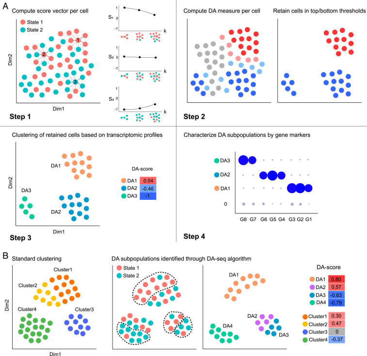
Fig. 1.

Schematic demonstration of DA-seq. (A) Illustration of the DA-seq algorithm. DA-seq detects DA subpopulations by analyzing cells from two biological states. The input of the algorithm is the union of data from two states after initial dimension reduction. Step 1: Computing a multiscale score vector, based on the $k$-nearest neighbors ($k$NN) of each cell, for several values of $k$ (e.g., $k=\mathrm{4,8,12}$). Step 2: Training a logistic classifier to predict the biological state of each cell based on the multiscale score to obtain a single DA measure. The algorithm retains only cells for which the DA measure is above a threshold ${\tau }_h$ or below ${\tau }_l$ and hence may reside in DA subpopulations. Step 3: Clustering the cells retained in step 2 to obtain contiguous DA subpopulations above a predefined size. These subpopulations are denoted $DA1$, $DA2$, and $DA3$. The degree of their differential abundance is quantified by a DA score (SI Appendix, Note 1). Step 4: Detect subsets of genes that characterize each of the DA subpopulations. For example, the genes G7 and G8 characterize $DA3$. (B) Standard clustering analysis vs. DA-seq. (Left) Cluster information obtained through standard clustering analysis. (Center) DA subpopulations identified through DA-seq. (Right) Normalized differential abundance of DA subpopulations and clusters, represented by DA score.