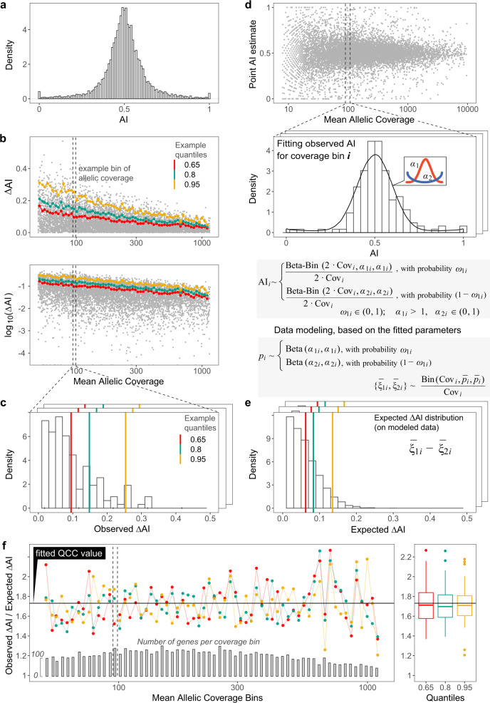
Fig. 3. Derivation of Quality Correction Coefficient from observed and modeled AI differences between technical replicates.
a–c Finding observed distributions of gene-level AI differences between replicates (ΔAI). a Distribution of point AI estimates for genes with allelic coverage over 10 in six pooled replicates (180M reads total) of Experiment 2. b Calculation of the observed distributions of AI differences between two replicates. After sampling an equal number of reads from two technical replicates, AI is calculated for each gene. Plotted is ΔAI against mean SNP coverage in linear (top) or log (bottom) scale. Genes are binned by log coverage (an example bin is shown). Quantiles are calculated per bin. Here and elsewhere, three example quantiles are shown: 0.65 (red), 0.8 (green), 0.95 (orange). c Distribution of the observed ΔAI values in a bin. Example quantiles are shown. d–e Calculation of the expected distributions of AI differences between replicates. d Top: AI for each gene is calculated after pooling SNP counts from both replicates. Note that we use mean SNP coverage, so the bins contain the same genes in both replicates. Bottom: For each coverage bin, distribution of AI values is fitted with a mixture of two symmetric beta-binomial distributions (red and blue curves). e Distribution of the expected ΔAI values in a bin. To generate expected ΔAI: we generate a simulated sample of 5000 genes, with the distribution of exact allelic imbalance values (ξ) according to the fitted parameters; from these genes, we then simulate two replicate datasets, with SNP coverage according to the bin, and sampling from binomial distribution; finally, we calculate the simulated ΔAI for each gene and find quantiles for their distribution. f Ratios of observed and expected values for the example ΔAI quantiles. Fitted black line defines Quality Correction Coefficient. Boxplots (right) summarize values for all coverage bins (left). Boxplot elements (right)--center line: median; box: upper and lower quartiles; whiskers: 1.5 x interquartile range; points: outliers.

