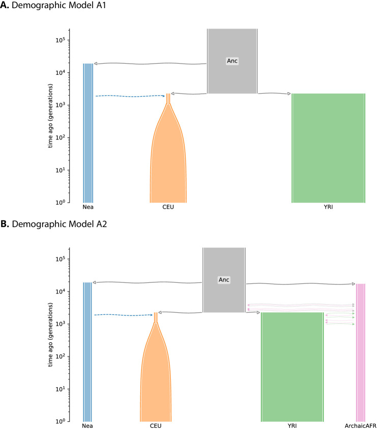
Figure 1. A schematic overview of how genomatnn detects adaptive introgression.

We first simulate a demographic history that includes introgression, such as Demographic Model A1 shown in (A), using the SLiM engine in stdpopsim. Parameter values for this model are given in Appendix 3—table 1. Three distinct scenarios are simulated for a given demographic model: neutral mutations only, a sweep in the recipient population, and adaptive introgression. The tree sequence file from each simulation is converted into a genotype matrix for input to the CNN. (B) shows a genotype matrix from an adaptive introgression simulation, where lighter pixels indicate a higher density of minor alleles, and haplotypes within each population are sorted left-to-right by similarity to the donor population (Nea). In this example, haplotype diversity is low in the recipient population (CEU), which closely resembles the donor (Nea). Thousands of simulations are produced for each simulation scenario, and their genotype matrices are used to train a binary-classification CNN (C). The CNN is trained to output Pr[AI], the probability that the input matrix corresponds to adaptive introgression. Finally, the trained CNN is applied to genotype matrices derived from a VCF/BCF file (D).

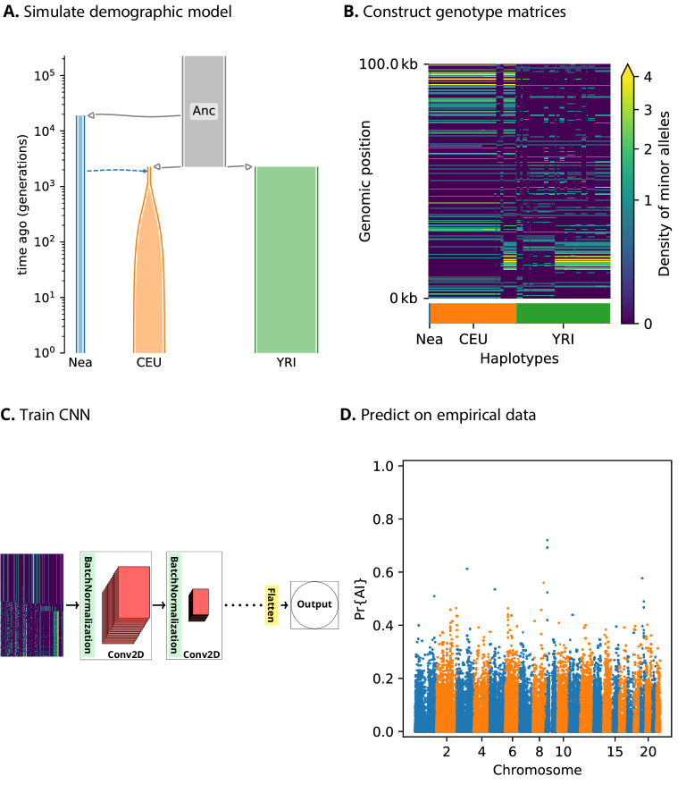
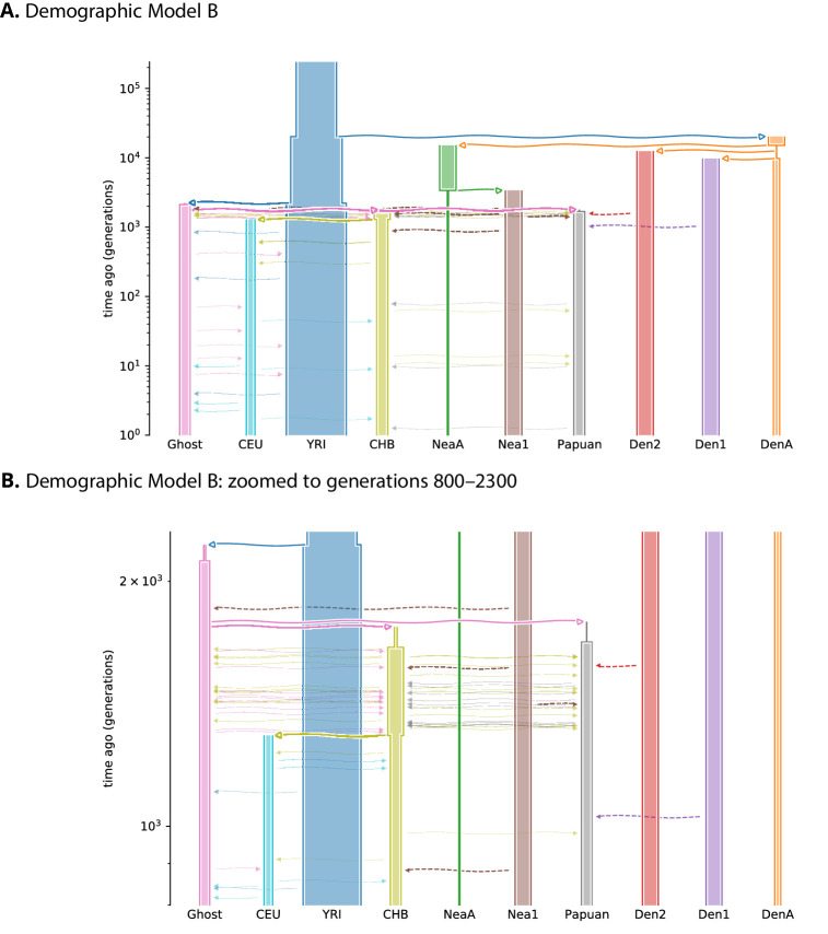
Figure 1—figure supplement 1. Schematic overview of Demographic Model A1 and A2.

Schematic overview of Demographic Model A1 (A) and A2 (B). Each population is depicted as a tube, where the tube’s width is proportional to the population’s size at any given time. Horizontal lines with arrows indicate either an ancestor/descendant relation (thick solid lines, open arrow heads), an admixture pulse (dashed lines, closed arrow heads), or a period of continuous migration (thin solid lines, closed arrow heads). The time of continuous migration lines were drawn randomly from the time interval over which the migrations occur. A Demes-format YAML file for each demographic model is available from the genomatnn git repository.

Figure 1—figure supplement 2. Schematic overview of Demographic Model B.

Overview of the Jacobs et al., 2019 demographic model (A), featuring two pulses of Denisovan gene flow into Papuans, which we implemented as the PapuansOutOfAfrica_10J19 model in stdpopsim. The same model is shown in (B), zoomed in to more clearly show the many events occurring between generations 800–2300. Each population is depicted as a tube, where the tube’s width is proportional to the population’s size at any given time. Horizontal lines with arrows indicate either an ancestor/descendant relation (thick solid lines, open arrow heads), an admixture pulse (dashed lines, closed arrow heads), or a period of continuous migration (thin solid lines, closed arrow heads). The time of continuous migration lines were drawn randomly from the time interval over which the migrations occur. DenA and NeaA are the sampled populations corresponding to Altai Denisovan and Altai Neanderthal, while Den1, Den2, and Nea1 correspond to introgressing lineages. A Demes-format YAML file for each demographic model is available from the genomatnn git repository.