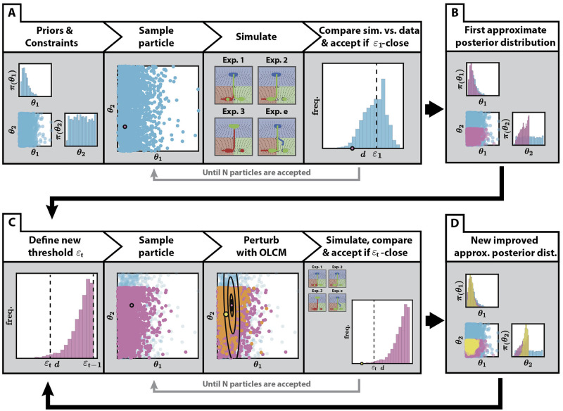
Fig 3. Application of ABC SMC to the fitting of the binary flip with cusp model.

(A) First step of the algorithm. Having defined priors for the fitted parameters and constraints between them, as well as an initial threshold ε₁, particles are sampled from the priors and accepted if the distance between the simulated data and the experimental data is less than the initial threshold. This is repeated until N particles are accepted. (B) An initial approximation of the posterior distribution is obtained, generated by the N particles accepted in (A). (C) The algorithm then proceeds in a sequential manner. In each step t of the algorithm, a new threshold ε_t is defined, in our case, the 0.3 quantile of the previous distribution of distances ε_t−1. Particles are sampled from the last approximate posterior distribution and perturbed using a Markov Kernel obtained from the Optimal Local Covariance Matrix (OLCM) [35] (black ellipses in the figure represent confidence intervals), (as described in S1 Appendix). This is repeated until N new particles that satisfy the distance threshold are accepted. Also, each new particle is assigned a weight proportional to its prior probability and inversely proportional to the Markov Kernels evaluated at this particle, which control for efficient exploration. (D) After each step, a new improved approximate posterior distribution is obtained, which restricts the values of the parameters to a restricted region of the parameter set.