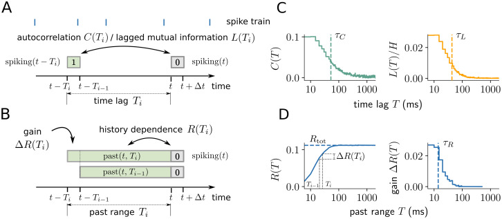
Fig 1. Illustration of history dependence and related measures in a neural spike train.
(A) For the analysis, spiking is represented by 0 or 1 in a small time bin Δt (grey box). Autocorrelation C(Ti) or the lagged mutual information L(Ti) quantify the statistical dependence of spiking on past spiking in a single past bin with time lag Ti (green box). (B) In contrast, history dependence R(Ti) quantifies the dependence of spiking on the entire spiking history in a past range Ti. The gain in history dependence ΔR(Ti) = R(Ti) − R(Ti−1) quantifies the increase in history dependence by increasing the past range from Ti−1 to Ti, and is defined in analogy to the lagged measures. (C) Autocorrelation C(T) and lagged mutual information L(T) for a typical example neuron (mouse, primary visual cortex). Both measures decay with increasing T, where L(T) decays slightly faster due to the non-linearity of the mutual information. Timescales τC and τL (vertical dashed lines) can be computed either by fitting an exponential decay (autocorrelation) or by using the generalized timescale (lagged mutual information). (D) In contrast, history dependence R(T) increases monotonically for systematically increasing past range T, until it saturates at the total history dependence Rtot. From R(T), the gain ΔR(Ti) can be computed between increasing past ranges Ti−1 and Ti (grey dashed lines). The gain ΔR(T) decays to zero like the time-lagged measures, with information timescale τR (dashed line).

