. 2021 May 5;10:e67784. doi: 10.7554/eLife.67784

Figure 3. Glucosinolate variation across Europe is dominated by two loci.

(A) The accessions are plotted on the map based on their collection site and colored based on their principal component (PC)1 score. (B) Manhattan plot of genome-wideassociation analyses using PC1. Horizontal lines represent 5% significance thresholds using Bonferroni (red) and Benjamini–Hochberg (blue).

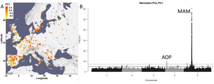
Figure 3.

Figure 3—figure supplement 1. Glucosinolate (GSL)-based principal component (PC) analysis.

Figure 3—figure supplement 1.

(A) Percentage of variance explained by each PC. (B, C) Contribution of the individual GSLs to PC1 (B) and PC2 (C). Red bars: contribution of four carbon GSLs; blue bars: contribution of three carbons GSLs. ± above the bar indicates if the contribution of the variable is positive or negative. (D) Linear model for PC1 and PC2 scores with the geographic parameters. Lat: latitude; Long: longitude.
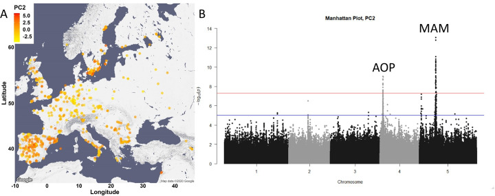
Figure 3—figure supplement 2. Glucosinolate variation across Europe is dominated by two loci.

Figure 3—figure supplement 2.

(A) The accessions were plotted on the map based on their collection site and colored based on their principal component (PC)2 score. (B) Manhattan plot of genome-wideassociation analyses using PC2. Horizontal lines represent 5% significance thresholds using Bonferroni (red) and Benjamini–Hochberg (blue).
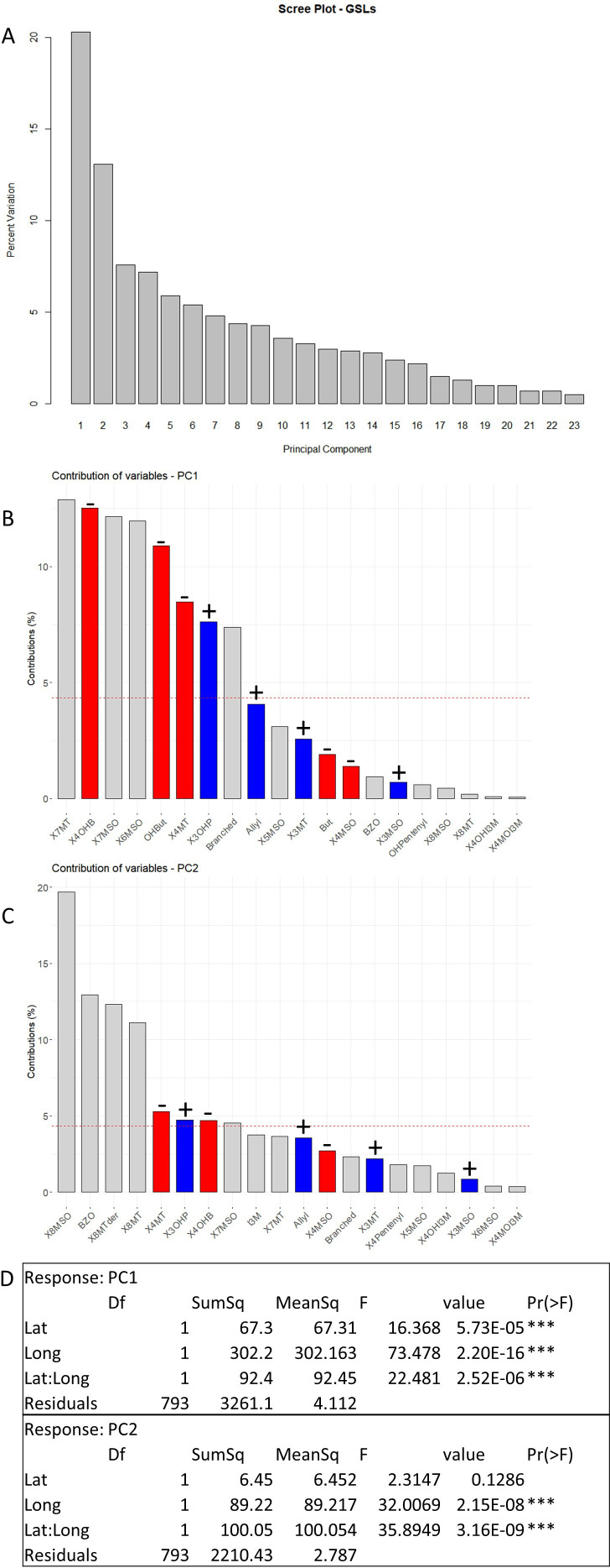
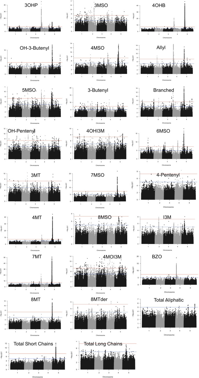
Figure 3—figure supplement 3. Manhattan plots of genome-wideassociation performed based on individual glucosinolate amounts as traits.

Figure 3—figure supplement 3.

Horizontal lines represent 5% significance thresholds using Bonferroni (red) and Benjamini–Hochberg (blue).