Extraction of rapid kinetics from smFRET measurements using integrative detectors

SUMMARY

Hidden Markov models (HMMs) are used to learn single-molecule kinetics across a range of experimental techniques. By their construction, HMMs assume that single-molecule events occur on slower timescales than those of data acquisition. To move beyond that HMM limitation and allow for single-molecule events to occur on any timescale, we must treat single-molecule events in continuous time as they occur in nature. We propose a method to learn kinetic rates from single-molecule Förster resonance energy transfer (smFRET) data collected by integrative detectors, even if those rates exceed data acquisition rates. To achieve that, we exploit our recently proposed “hidden Markov jump process” (HMJP), with which we learn transition kinetics from parallel measurements in donor and acceptor channels. HMJPs generalize the HMM paradigm in two critical ways: (1) they deal with physical smFRET systems as they switch between conformational states in continuous time, and (2) they estimate transition rates between conformational states directly without having recourse to transition probabilities or assuming slow dynamics. Our continuous-time treatment learns the transition kinetics and photon emission rates for dynamic regimes that are inaccessible to HMMs, which treat system kinetics in discrete time. We validate our framework’s robustness on simulated data and demonstrate its performance on experimental data from FRET-labeled Holliday junctions.

Graphical Abstract

Kilic et al. apply their recently developed HMM generalization toward unraveling single-molecule FRET kinetics occurring on timescales exceeding data acquisition rates of integrative detectors. This HMM generalization treats single-molecule kinetics in continuous time, as occurs in nature, and treats integrative-detector measurements as occurring in discrete time.

INTRODUCTION

Fluorescence experiments based on single-molecule Förster resonance energy transfer (smFRET) can probe the switching kinetics between conformational states defined by different inter- and intra-molecular distances.^1–7 In a prototypical intra-molecular smFRET experiment, one portion of a molecule of interest is attached to a donor fluorophore and another to an acceptor fluorophore.^1–15 In such experiments, the excitation wavelength is most commonly adjusted to excite the donor,^6,11,13–15 and for a donor sufficiently far from the acceptor, the donor is excited and emits shorter wavelength light as compared with the longer wavelength light emitted by the acceptor in the case of energy transfer when a donor and acceptor are in proximity.^6,11,13–15 Because of the difference in the wavelength of light emitted by donors and acceptors, photons emitted are registered across different detectors.^6,11,13–15 We refer to the recordings in the two detectors as the donor and acceptor channels.^6,11,13–15 As such, the sequence of photon detection² encodes the kinetics; according to which, the distance varies between both fluorophores down to microsecond timescales.^1–6 Existing approaches for analyzing smFRET data include FRET efficiency histogram-based methods, although such methods discard the important temporal information encoded in donor and acceptor photon arrival sequences.^{4–6,8–10,12,13,16} What is more, FRET efficiency histogram analysis is difficult to generalize beyond two conformational states.¹⁷ In addition, because arbitrary binning is required to construct histograms, such methods often lead to inconclusive or erroneous estimates.^4,18–20 For these reasons, modeling efforts have moved toward more direct time-series analyses.^5,17,21–24

By relying on the hidden Markov model (HMM) paradigm,^{1,3,5,23,25–32} time series analysis fully considers the temporal arrangement (i.e., the sequence) of photon detections and avoids histogram binning artifacts.^1,3,5,25 This paradigm is especially fruitful in analyzing demanding experiments, such as conformational states, which are treated as the hidden states of the HMMs, are themselves indirectly observed because of shot noise,^1,3 and also allows for inclusion of measurement noise and specialized detector characteristics in the analysis.^1,3,5,25

Starting with Ref.¹² and later with others,^{1,3,5,23,28,33} HMMs and their variants have had important assumptions built into them. Those are the assumptions we wish to remove in an effort to analyze conformational transitions occurring on timescales faster than the data acquisition rate 1/Δt supported by integrative detectors, such as cameras. Before describing these assumptions, we discuss Δt (the bin size for photon collection), otherwise known as the frame rate or temporal resolution. Because Δt is determined mostly by the integrative detectors, for simplicity, we assume that the same Δt applies to both channels.

To learn rates that exceed data-acquisition rates, the most critical HMM assumptions we need to remove are the following:

• HMMs make the assumption that the state switches occur rarely as compared to Δt. In other words, all switching rates are assumed to be much slower than 1/Δt. For that reason, HMMs are formulated using transition probabilities rather than transition rates.

• HMMs approximate the transitions as occurring precisely at the end of each data acquisition period.^{23,28,34–39} In other words, intra-frame motion does not occur. For that reason, HMMs represent only instantaneous states and measurements.

The first assumption is particularly relevant to the present study because it requires, before an analysis, that all transitions be slower than Δt. In general, this is not only unknown but also difficult to assess beforehand. After all, the objective of many experiments is to determine the switching rates, in the first place. The second assumption is also relevant to the present study because, before an analysis, it needs to balance two competing requirements: an upper bound on Δt set by the fastest switching rate, and a lower bound on Δt supported by the detection hardware.

One method, termed H²MM (a variant of HMM), was specifically developed to overcome these challenges.³ In H²MMs, HMMs are applied on time grids finer than the measurement time interval. However, because of the finer grid, H² MMs and their variants suffer from high computational costs.⁴⁰ For that reason, continuous time formulations,^40,41 which allow transitions to occur at any time, have been sought. Formulations such as those are important because they would provide a framework to develop robust and general methods for extracting kinetics that are faster than the data acquisition time and may provide ways to improve on previous efforts to extract fast kinetics, which have been limited in various ways, e.g., limited to two conformational states.³¹ In particular, an important goal of ours herein is to adapt continuous-time formulations^40,41 to the averaging inherent to integrative detector modalities.

We mention in passing that alternate approaches have been developed to analyze fast kinetics by smFRET,^1,9,42,43 although they have been tied to the analysis of single-photon arrivals. Such methods do not rely on the HMM paradigm because they do not analyze binned data collected by integrative detectors, even though those methods are also limited by the photon detection rate. As such, they do not suffer from the limitations of HMMs.

However, all the aforementioned methods, whether in the analysis of single-photon data or binned data,^1,3,9,42,43 rely on maximum likelihood,⁴⁴ often with assumptions required to render computations analytically tractable (such as assuming there are only transitions between two linearly arranged conformational states).⁴⁵ Because of working within a maximum-likelihood approach, only point estimates of the quantities of interest can be directly drawn from the data with additional statistical strategies, such as Fisher information or bootstrapping, used to extract error bars.⁴⁴

Maximum-likelihood methods lie in sharp contrast to the Bayesian methods we will employ, which will allow us to directly propagate measurement uncertainty into an uncertainty over parameter estimates.

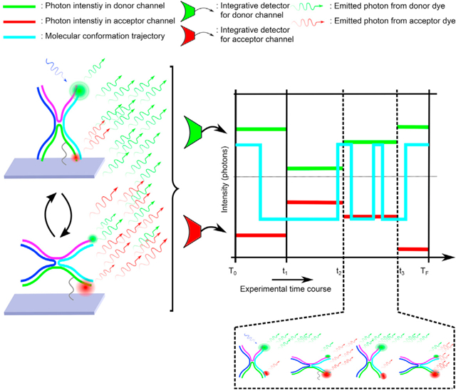
In Figures 1A and 1C, we illustrate an example of smFRET measurements acquired with integrative detectors, such as modern scientific-grade cameras. In Figure 1A, we show an example with slow kinetics (relative to Δt). These data are primarily contaminated with shot noise and can be reliably analyzed within the HMM paradigm. In contrast, in Figure 1C, we demonstrate an example with fast kinetics (relative to Δt). In addition to shot noise, these data are contaminated with significant intra-frame transitions; consequently, they cannot be analyzed within the HMM paradigm. As the molecule undergoes fast switching between the states during the data-acquisition period, the measurement associated with that period reports on the average signal from the molecule over that period, and the state of the molecule cannot be deduced from a model operating exclusively on instantaneous states, such as within the HMM paradigm. Nonetheless, the information on fast switching is itself encoded within that measurement, even though some of the information is indeed lost. It is, therefore, necessary to develop a method that can accommodate continuously evolving dynamics to learn the kinetics from the measurements, instead of invoking an HMM formulation that, by construction, violates that critical feature.

Figure 1. An illustration of single molecule switching kinetics and corresponding measurements.

(A–D) We provide the simulated trajectory (cyan) of the single molecule between two states(σ₁ and σ₂) (A and B). The photon emission rates, i.e., the number of emitted photons per unit of time in the absence of noise in both donor and acceptor channels, associated with the conformation states σ₁ andσ₂, are labeled with ${\mu }_{{\sigma }_1}$ and ${\mu }_{{\sigma }_2}$, respectively. The simulated experiment provided in this figure starts at Δt = 0.05 s and ends at t_N = 10 s with the data acquisition period being Δt = 0.05 s. Here, in (A) and (C), for visual purposes, we assume that the measurements are acquired by a detector with a fixed exposure period of τ = 50 ms in donor (green) and acceptor (red) channels. As the molecule switches between states (σ₁ and σ₂) during an integration period, the measurements represent the number of total emitted photons and reflect the rates ${\mu }_{{\sigma }_1}$, ${\mu }_{{\sigma }_2}$, which correspond to the visited conformational states. (A) and (B) represent the simulated data in which the molecule-switching kinetics between the conformation states are slower than the data acquisition rate. On the other hand, in (C) and (D), we demonstrate a single-molecule trajectory (cyan) when the molecule’s switching kinetics are faster than the data acquisition rate. In (B), the slow kinetics of the molecule give rise to well-separated state-occupancy histograms in donor and acceptor channels around the average photon emission rates. By contrast, in (D), we don’t observe well-separated histograms because of the fast-switching kinetics of the molecule.

To achieve that, a new method needs to (1) represent the dynamics of the molecule in continuous time, (2) model the acquired measurements at each data acquisition times via the average dynamics of the molecule within the associated data-acquisition period, and (3) entail manageable computational cost so it allows for practical applications and propagation of errors from measurement uncertainty.

For this reason, we now turn to Markov jump processes (MJPs), which describe continuous time dynamics,^46–50 and propose inference strategies for the MJPs.^40,41,51

The focus of this work is to adapt inverse strategies on MJPs to deal with the integrative nature of the detectors (that average smFRET signal over the exposure windows) to extract fast kinetics. Because we extract MJPs hidden by the integrative nature of the measurement, we call our method the hidden MJP (HMJP). As we will see, HMJPs are direct generalizations of HMMs, and as such, HMJPs will rigorously reduce to the HMM as the exposure period approaches zero, Δt→0.

Briefly, in the results section, we provide HMM and HMJP analysis comparisons on simulated measurements of smFRET collected by integrative detectors. In comparing the HMM and HMJP, we present their respective performance in acquiring photon-emission rates, transition probabilities (for HMMs), and kinetic rates (for HMJPs). We demonstrate how HMJPs successfully outperform HMMs, especially for fast kinetic rates, as compared with the data-acquisition rate. Their comparison on slow-switching kinetics of simulated smFRET data (in which both the HMM and HMJP, as expected, do well) can be found in supplemental information. Subsequently, we move onto the analysis of experimental data. We provide a comparison of HMJPs and HMMs in their learning of molecular trajectories, transition probabilities, and kinetic rates. Next, in our discussion, we describe the broader potential for HMJPs for smFRET applications. Lastly, in our experimental procedures section, we provide our HMJP smFRET model description and briefly, for sake of comparison, summarize plain HMMs for smFRET applications.

RESULTS

Simulated data analysis overview

To show how HMJPs work and to highlight the advantages of HMJPs over that of HMMs, we initially benchmark our method using simulated data that mimics smFRET experiments. Simulated data are ideal for this purpose because they have a “ground truth.” Generation of such data relies on the Gillespie algorithm.⁵² Next, we compare the strength of our HMJP method to that of HMMs on experimental data.

We focus on the following simulated datasets: a molecule exhibiting fast kinetics, as compared with the data-acquisition rate, and with two and three conformational states (see Figures 1 and 2, respectively).

Figure 2. An illustration of experimental smFRET measurements for data acquisition periods Δt = 0.05 s.

(A and B) We provide the measurements for the simulated trajectory of the single molecule between three states (σ₁, σ₂, and σ₃) with the same color scheme as shown in Figure 1 (A). Here, we assume that the measurements are acquired by integrative detectors with fixed exposure periods that coincide with a data acquisition period of τ = 0.05 s in the donor (green) and acceptor (red) channels.

The simpler analysis of datasets with slow kinetics can be found in supplemental information. The results corresponding to the simulated dataset with fast kinetics for both HMJP and HMM are shown in Figures 3 and 4. Subsequently, we show the performance of our method on an experimental dataset (Figure 5). We present the results for the experimental dataset in Figures 6, 7, 8, and 9. Further analysis on different experimental datasets, additional analysis of datasets with more than two conformational states, and an analysis of simulated datasets generated based on electron multiplying charge-coupled device (EMCCD)⁵³ models are also provided in supplemental information.

Figure 3. The HMJP and HMM photon emission rate, escape rate, and transition-probability estimates for fast-switching kinetics in simulated measurements.

(A and B) Here, we provide the posterior photon emission rate, escape rate, and transition-probability estimates obtained with HMJP and HMM when the switching rate is faster than the data acquisition rate 1/Δt = 20 (1 /s). We expect HMMs to perform poorly in estimating the true photon emission rates, escape rates, and transition probabilities when the system switching is fast. In (A) and (B), we superposed the posterior distributions over photon emission rates for HMJP (green for donor, orange for acceptor) and HMM (blue for donor, pink for acceptor) along with their 95% confidence intervals (also known as credible intervals) and the true photon emission rates (cyan line).

(C–F) We superposed the posterior distributions over the escape rates and transition probabilities (green for HMJP and blue for HMM) along with their 95% confidence intervals, true escape rates, and true transition probabilities (cyan lines), respectively. (C) and (D) correspond to the posterior distribution of the escape rates that are labeled with ${\lambda }_{{\sigma }_k}\to {\sigma }_{k^{\prime }}$ for all k, k′ = 1, 2 with k ≠ k′. (E) and (F) correspond to the transition probabilities labeled as $P_{{\sigma }_k}\to {\sigma }_k$ for allk = 1, 2. Here, simulated measurements are generated with the same parameters as those provided in Figures 1C and 1D.

Figure 4. HMJP and HMM photon emission rate, escape rate and transition probability estimates for fast switching kinetics in simulated measurements for 3 conformational states.

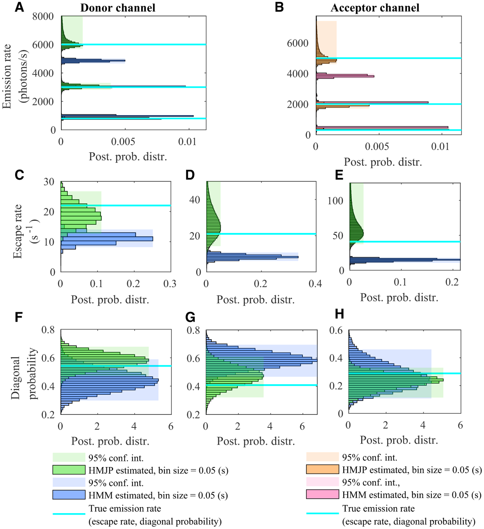
(A–H) Here, we provide posteriors over the photon emission rate, escape rate, and transition-probability estimates obtained with HMJPs and HMMs when the switching rate is faster than the data acquisition rate 1/Δt for three conformational states. We expect HMMs to perform poorly in estimating the true photon emission rates, escape rates, and transition probabilities when the system switching is fast. Here, we provide the posterior distributions with the same color convention as in Figure 3. Simulated measurements used here are generated with the same parameters as those provided in Figures 2A and 2B.

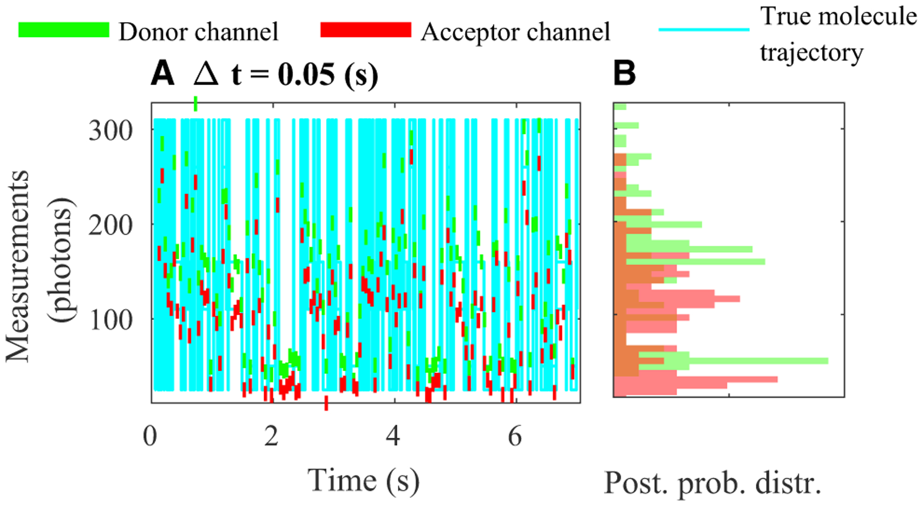
Figure 5. An illustration of experimental smFRET measurements for data acquisition periods Δt = 0.025 s, Δt = 0.05 s, and Δt = 0.1 s.

(A–F) In (A), (C), and (E), we provide the measurements for the same smFRET experiment coinciding with the data acquisition periods Δt = 0.025 s, Δt = 0.05 s, and Δt = 0.1 s. Here, we assume that the measurements are acquired by detectors with fixed exposure periods coinciding with the data acquisition periods τ = 0.025 s, τ = 0.05 s, and τ = 0.1 s in donor (green) and acceptor (red) channels. (B), (D), and (F) are especially interesting to our analysis. Here, we don’t observe well-separated histograms because of the fast-switching kinetics of the molecule, as shown in Figure 1D for simulated experiments.

Figure 6. HMJP and HMM photon emission rate, escape rate and transition probability estimates for experimental smFRET measurements with Δt = 0.025 s.

(A–F) Here, we provide posterior photon emission rate (A and B), escape rate (C and D), and transition probability (E and F) estimates obtained with HMJP and HMM for the experimental data shown in Figure 5A. Here, we follow a similar color convention to that of Figure 3. However, unlike Figure 4, ground-truth information is not available for the photon emission rates, escape rates, and transition probabilities because the analysis is performed with experimental data.

Figure 7. HMM photon emission rate, escape rate and transition probability estimates for experimental smFRET measurements with Δt = 0.025 s, Δt = 0.05 s, and Δt = 0.1 s.

Here, we provide posterior photon emission rate, escape rate, and diagonal transition-probability estimates obtained with HMM for the measurements shown in Figures 5A, 5C, and 5E. We do not expect HMM posterior estimates associated with three different exposure periods to be consistent because of the switching-kinetics approach for the data acquisition rate.

(A and B) We superposed the posterior distributions for the measurements associated with exposure periods Δt = 0.025 s, Δt = 0.05 s, and Δt = 0.1 s over the photon emission rates for HMM, along with their 95% confidence intervals.

(C and D) We superposed the posterior distributions over the escape rates along with their 95% confidence intervals.

(E and F) We superposed the posterior distributions over transition probabilities and their 95% confidence intervals. Posterior distributions over photon emission rate, escape rate, and diagonal transition probability estimates for the integration periods Δt = 0.025 s, Δt = 0.05 s, and Δt = 0.1 s are demonstrated in green, blue, and purple, respectively.

Figure 8. HMJP photon emission rate, escape rate and transition probability estimates for experimental smFRET measurements with Δt = 0.025 s, Δt = 0.05 s, and Δt = 0.1 s.

Here, we provide posterior photon emission rate, escape rate, and diagonal transition probability estimates obtained with HMJP for the measurements shown in Figures 5A, 5C, and 5E. We expect HMJP posterior estimates associated with three different exposure periods to be consistent across examples, even if the switching kinetics exceed data acquisition rate.

(A and B) We superposed the posterior distributions for the measurements associated with exposure periods Δt = 0.025 s, Δt = 0.05 s, and Δt = 0.1 s over the photon emission rates for the HMJP along with their 95% confidence intervals.

(C and D) We superposed the posterior distributions over the escape rates along with their 95% confidence intervals.

(E and F) We superposed the posterior distributions over transition probabilities and their 95% confidence intervals. Here, we follow a similar color convention as that in Figure 7.

Figure 9. HMM and HMJP FRET efficiency estimates for experimental smFRET measurements with Δt = 0.025 s, Δt = 0.05 s, and Δt = 0.1 s.

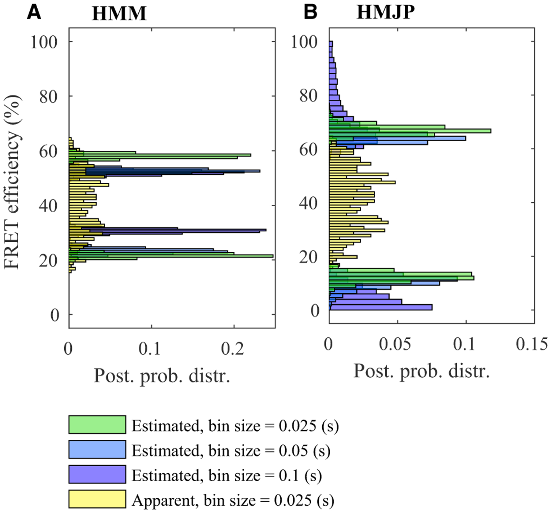
(A and B) Here, we provide posterior FRET efficiency estimates obtained with HMM and HMJP for the measurements shown in Figures 5A, 5C, and 5E. We expect inconsistent posterior FRET efficiency estimates for HMMs associated with three different exposure periods (A). On the other hand, we expect HMJPs to provide consistent posterior estimates over FRET efficiencies for three different exposure periods (B). Here, in (A) and (B), we superposed the posterior distributions over the FRET efficiencies along with the apparent FRET efficiency (yellow). In this figure, we follow a similar color convention to that used in Figure 7.

Hyperparameter values used in all analyses, as well as any other choices made, are presented in supplemental information. For clarity, we only have access to the data demonstrated with the green and red dashes of Figures 1A and 1C (not the cyan [ground truth] trajectories). Those ground truth trajectories are unknown and are determined along with other model parameters.

Acquisition of simulated data

In the generation of our simulated data, provided in Figure 1C, we assumed K = 2 attainable states, indexed as σ₁ and σ₂. These could be folded or unfolded states for illustrative purposes (our method trivially generalizes to more states).

We assumed photon emission rates indexed with ${\mu }_{{\sigma }_k}^D$ and ${\mu }_{{\sigma }_k}^A$ for the donor and acceptor in each attainable state σ_k, which we set to ${\mu }_{{\sigma }_1}^D=800\text{photons/s}$, ${\mu }_{{\sigma }_2}^D=\text{2000}\text{photons/s}$, and ${\mu }_{{\sigma }_1}^A=300\text{photons/s}$, and ${\mu }_{{\sigma }_2}^A=700\text{photons/s}$ where the background photon emission rates are set to ${\mu }_{\text{back }}^D={\mu }_{\text{back }}^A=200\text{photons/s}$ photons/s. Additionally, we defined a data-acquisition period of Δt = 0.05 and consider the exposure period by setting τ equal to 100% of Δt. The onset and concluding time of the simulated data are at t₀ = 0.095s and t_N = 10.05 s, respectively.

We use the parameter τ_f, as follows, to set a timescale in expressing the switching rates between both states $\left({\lambda }_{{\sigma }_1\to {\sigma }_2},{\lambda }_{{\sigma }_2\to {\sigma }_1}\right)$,

$${\lambda }_{{\sigma }_1\to {\sigma }_2}=\frac{2.2}{{\tau }_f},{\lambda }_{{\sigma }_2\to {\sigma }_1}=\frac{2.1}{{\tau }_f}$$ (Equation 1)

in the analysis of fast and slow switching rates.

We simulate the case with τ_f = 0.1 s in Figure 1C, which involves system kinetics exceeding the data acquisition rate. These kinetic rates are chosen to simulate data closer to the experimental data (shown later in Figure 5) to benchmark our framework.

In this simulated data, we set the data acquisition period to Δt = 0.05 s, such that our ${\lambda }_{{\sigma }_1\to {\sigma }_2}$ and ${\lambda }_{{\sigma }_2\to {\sigma }_1}$ exceed the data acquisition rate (1 /Δt).

Next, we simulated a dataset with fast dynamics (Figure 2), in which K = 3 attainable states (indexed σ₁ to σ₃) were assumed for the underlying dynamics of the single molecule. Further, we set photon emission rates for the donor and acceptor in each state as ${\mu }_{{\sigma }_1}^D=800\text{photons/s}$, ${\mu }_{{\sigma }_2}^D=3\text{00}\text{photons/s}$, ${\mu }_{{\sigma }_1}^D=6000\text{photons/s}$, ${\mu }_{{\sigma }_1}^A=300\text{photons/s}$, ${\mu }_{{\sigma }_2}^A=2000\text{photons/s}$, and ${\mu }_{{\sigma }_1}^A=5000\text{photons/s}$, where ${\mu }_{\text{back }}^D={\mu }_{\text{back }}^A=200\text{photons/s}$. The data acquisition period here was also set to Δt = 0.05 with the exposure period τ set to 100% of the data acquisition period. In the dataset demonstrated in Figure 2, the onset of the simulated experiment is t₀ = 0 s, where the final time is t_N = 7 s. The switching rates used in the generation of the dataset in Figure 2 are

$${\lambda }_{{\sigma }_1\to {\sigma }_2}=\frac{2.2}{{\tau }_f},{\lambda }_{{\sigma }_1\to {\sigma }_3}=0,{\lambda }_{{\sigma }_2\to {\sigma }_1}=\frac{2.1}{{\tau }_f},{\lambda }_{{\sigma }_2\to {\sigma }_3}=0,{\lambda }_{{\sigma }_3\to {\sigma }_1}=\frac{2}{{\tau }_f},{\lambda }_{{\sigma }_3\to {\sigma }_2}=\frac{2.1}{{\tau }_f}$$ (Equation 2)

with τ_f = 0.1 s.

Comparison of HMJPs with HMMs on simulated data

Here, we compare HMJPs and HMMs on the analysis of simulated measurements given in Figures 1C and 2A.

We start with the analysis of the data provided in Figure 1C. We expect HMJPs to perform better than HMMs do because the simulated data are generated with switching rates 5% faster than the data acquisition rate (and thus many transitions occur during the data acquisition time). In this regime of switching rates, the approximation in Equation 16 required by HMMs fails.

Given the measurements, we estimate the posterior distribution over the quantities of interest, including the trajectory, $\mathcal{T}(·)$; initial transition probability matrix, $\overline{\rho }$; transition probabilities $\overline{\overline{\pi }}$ (and $\overline{\overline{P}}$ in HMM); photon emission rates; ${\overline{\mu }}^D$, ${\overline{\mu }}^A$; and escape rates, $\overline{\lambda }$. To achieve these estimates, we use HMJP and HMM samplers as introduced in Computational inference section to generate pseudorandom numbers from the posterior distributions $\mathbb{P}\left(\overline{\rho },\overline{\overline{\pi }},\overline{\lambda },{\overline{\mu }}^D,{\overline{\mu }}^A,(\overrightarrow{S},\overrightarrow{D},M)\mid w^D,w^A\right)$ and $\mathbb{P}\left(\overline{\rho },\overline{\overline{P}},\overline{\mu },\overrightarrow{c}\mid w^D,w^A\right)$, respectively.

We first show emission and escape rate estimates in Figure 3. In Figures 3A–3F, we observe that the ground truths for photon emission rates, escape rates, and transition probabilities lie within the 95% confidence intervals for the corresponding HMJP estimates. For clarity, we compute the 95% confidence interval using only samples produced after burn-in. By contrast, the HMM performs poorly because of the failure of the approximation in Equation 16, resulting in an unsatisfactory photon emission rate and unsatisfactory escape rate estimates.

In particular, from Figures 3A and 3B, we see that the HMM overestimates ${\mu }_{{\sigma }_1}^D$ and ${\mu }_{{\sigma }_1}^A$ (by about 12%, namely, HMM provides estimates that are approximately 1.12 times the ground-truth values for ${\mu }_{{\sigma }_1}^D$ and ${\mu }_{{\sigma }_1}^A$) and underestimates (by about 5%) ${\mu }_{{\sigma }_2}^D$ and ${\mu }_{{\sigma }_2}^A$.

The failure of the HMM is more pronounced when looking at ${\lambda }_{{\sigma }_1}$ and ${\lambda }_{{\sigma }_2}$. For example, in Figures 3C and 3D, the HMM provides narrow distributions over escape rates by grossly underestimating both ${\lambda }_{{\sigma }_1}$ and ${\lambda }_{{\sigma }_2}$ (by about 50%). On the other hand, in Figures 3C and 3D, we see that HMJP posterior distribution mode coincides with the ground truth.

The HMM inability to capture fast kinetics is also reflected by its wide posterior distributions over transition probabilities $P_{{\sigma }_1\to {\sigma }_1}$, $P_{{\sigma }_2\to {\sigma }_2}$ as shown in Figures 3E and 3F.

We next move to the analysis of the data provided in Figure 2A. Just as with the analysis of Figure 1C, we observe similar results in Figure 4. In particular, from Figures 4A and 4B, we observe that HMMs fail to estimate ${\mu }_{{\sigma }_1}^D$, ${\mu }_{{\sigma }_1}^A$, ${\mu }_{{\sigma }_3}^D$, and ${\mu }_{{\sigma }_3}^A$, such that the HMMs overestimate (by about 30%) ${\mu }_{{\sigma }_1}^D$ and ${\mu }_{{\sigma }_1}^A$. whereas they underestimate (by about 20%) ${\mu }_{{\sigma }_3}^D$ and ${\mu }_{{\sigma }_3}^A$. By contrast, the mode of the HMJP posterior over photon emission coincides with the ground truth for both donor and acceptor channels. Next, HMMs provide broad, uncertain transition-probability estimates as shown in Figures 4F–4H. These poor HMM transition probability estimates give rise to the tight posterior escape rate estimates shown in Figures 4C–4E, based on Equation 16. By contrast, the HMJP posteriors over transition probabilities, as well as escape rates, have modes coinciding with the ground truths.

In supplemental information and Figure S1, we provide an analysis of slow-switching kinetics for the HMJP and HMM estimate comparisons shown in Figure 3, where both HMJP and HMM perform well.

Subsequently, in supplemental information and Figure S2, we provide the robustness of HMJP posterior estimates over photon emission rates, escape rates, and transition probabilities for the dataset provided in Figure 1C. We observe that, when the kinetic rates are more than four times the data acquisition rate, the HMJP starts failing in providing consistent posterior estimates over photon emission rates, escape rates, and transition probabilities. We have run further analyses to test the HMJP performance in estimating posterior distributions for photon emission rates and switching rates on the data generated for five cases.

First, we considered fast dynamics and different exposure periods (see Figures S3 and S4). In this first case, we tested the robustness of the HMJP framework on a two-state system in estimating photon emission rates and switching rates in which the ground-truth switching rates differ by more than the ones used to generate the data shown in Figure 1. In addition, we performed this test for the estimates of the HMJP for two different exposure periods. We demonstrate in Figures S3 and S4 that the HMJP posteriors over photon emission rates and switching rates have ground-truth values that lie in the posterior’s 95% confidence intervals.

Second, we generated data with slow-fast (in which we have mixed regime of few or many transitions occurring within a data acquisition period) dynamics and different exposure periods (see Figures S5 and S6). Here, we run the same test as presented in the first case but for switching kinetics, and we observe both slower and faster kinetics for the simulated single molecule than the data acquisition rate. The HMJP still performed well in estimating both photon emission rates and switching kinetics (see Figures S5 and S6).

Third, we generated data with fast dynamics by using three different sets of photon emission rates (see Figures S7–S9). Here, we tested the robustness of HMJP in estimating posterior photon emission rates and switching kinetics for various differences in photon emission rates across each conformational states of the simulated single-molecule trajectory. In this test, the HMJP still performed quite well in estimating photon emission rates and switching kinetics when the switching kinetics exceeded the data acquisition rate on datasets generated with a range of photon emission rates.

Fourth, we tested the HMJP on its ability to deduce the correct parameters when an incorrect model is specified. For example, we specified three states for data generated using two states and found that the additional state learned was redundant (see Figures S10–S12).

Fifth, we tested the performance of our model on data simulated using a specific time for the integrative detector (EMCCDs).⁵³ We have run our analysis on simulated data generated with three conformational state dynamics. Further, we set photon emission rates for donor and acceptor at ${\mu }_{{\sigma }_1}^D=800\text{photons/s}$, ${\mu }_{{\sigma }_2}^D=3\text{000}\text{photons/s}$, ${\mu }_{{\sigma }_3}^D=6000\text{photons/s}$, and ${\mu }_{{\sigma }_1}^A=300\text{photons/s}$, ${\mu }_{{\sigma }_2}^A=2000\text{photons/s}$, and ${\mu }_{{\sigma }_3}^A=5000\text{photons/s}$, where ${\mu }_{\text{back }}^D={\mu }_{\text{back }}^A=200\text{photons/s}$. The data acquisition period here was also set to Δt = 0.05 s with the exposure period τ set to 100% of the data acquisition period. In the dataset demonstrated in Figure S13, the onset of the simulated experiment is t₀ = 0 s where the final time is t_N = 7 s. The switching rates used in the generation of the dataset in Figure S13, used τ_f = 0.1 s and

$${\lambda }_{{\sigma }_1\to {\sigma }_2}=\frac{1}{{\tau }_f},{\lambda }_{{\sigma }_1\to {\sigma }_3}=\frac{1.2}{{\tau }_f},{\lambda }_{{\sigma }_2\to {\sigma }_1}=\frac{1.5}{{\tau }_f},{\lambda }_{{\sigma }_2\to {\sigma }_3}=\frac{0.6}{{\tau }_f},{\lambda }_{{\sigma }_3\to {\sigma }_1}=\frac{1}{{\tau }_f},{\lambda }_{{\sigma }_3\to {\sigma }_2}=\frac{0.5}{{\tau }_f}.$$ (Equation 3)

We presented the results for the posterior switching-rate estimates and the photon emission rates in donor and acceptor channels in Figures S14–S16, respectively. We observe that our framework performs very well in estimating the model parameters in the case of a different camera model along with fast-switching dynamics based on the provided posterior estimates. We now move onto the analysis of experimental datasets.

Experimental data analysis overview

Having benchmarked our HMJP on the simulated smFRET dataset, we now move on to assessing the HMJP performance on experimental smFRET data provided in Figure 5, for Holliday junctions (HJs), as described in the sample preparation. We deliberately start from single photon arrival datasets. Such datasets give us the flexibility to bin data as we please to mimic experimental data collected over a broad range of binning conditions as is the case in several studies.^4,18–20 In particular, we bin using three data acquisition periods: Δt = 0.025s (with results shown in Figures 6, 7, 8, and 9), Δt = 0.05s (with results shown in Figures 6, 7, 8, and 9), and Δt = 0.1 s (with results shown in Figures 6, 7, 8, and 9). We picked these bin sizes for a particular reason: we estimate rates of ~35–45 (1/s) for the smallest bins. Then, we consider data acquisition rates that are twice and four times larger. We also set the exposure period, τ to 100% of the Δt, namely, τ = 0.025, 0.05 s and τ = 0.1 s.

We emphasize that the fast transitions are averaged away when the data acquisition period is larger, especially for Δt = 0.1 s (in other words, when we have the largest time bin provided in Figure 5E). Thus, the largest time bin may, counter-intuitively, appear as though it had the best separated peaks (see the histograms in Figure 5). However, despite being the sharpest, it has the least amount of information.

As we will see, the HMJP returns values for the rates that are consistent across bin sizes, as would be expected for a method that can learn transition rates slower or faster than the data-acquisition rate. By contrast, the failure of HMM becomes apparent because of the inconsistency of the estimates for the switching kinetics as a function of the data bin size. The HJs we used have two well-characterized conformational states.^3,54 Here, our goal was to estimate the HJ emission and switching rates, in addition to the trajectory of HJs, simultaneously.

In Figures 5A, 5C, and 5E, we show the data under all three different bin sizes. From the data, we estimate the posterior distribution over the trajectory, $\mathcal{T}(·)$; initial transition probability matrix, $\overline{\rho }$; transition probabilities, $\overline{\overline{\pi }}$ (and $\overline{\overline{P}}$ in HMM); photon emission rates, ${\overline{\mu }}^D$, ${\overline{\mu }}^A$; and escape rates, $\overline{\lambda }$. In Figure 6, we show a direct comparison of the HMJP and HMM under the smallest bin size, in which we anticipate both HMM and HMJP to be consistent with one another. As we move to larger bin sizes, the HMJP remains consistent with the results that we obtained for the smallest bin, but the HMM eventually shows a lack of consistency as the bin sizes increase. This is apparent from Figure 7, in which we look at the increasing bin size for HMM, and in Figure 8, in which we look at the increasing bin size for HMJP. Finally, in Figure 9, we show the estimates over FRET efficiencies, in which we increase bin sizes for both HMM and HMJP.

Comparison of HMJPs with HMMs on experimental data

We begin with an HMJP and HMM comparison for the smallest bin size, Δt = 0.025s (see Figure 5A), on the photon emission rates, escape rates, and transition probability estimates provided in Figure 6. We show that the simulated dataset provided in Figure 1 mimics the dataset provided in Figure 5.

Even though, for experimental data shown in Figure 5A, the “ground truth” photon emission rates, escape rates, and transition probabilities are not known, we suspect that similar observations provided in Figure 3 hold for those in Figure 6.

In Figures 6A and 6B, we observe that HMM overestimates ${\mu }_{{\sigma }_1}$ and underestimates ${\mu }_{{\sigma }_2}$ compared with HMJP estimates for ${\mu }_{{\sigma }_1}$ and ${\mu }_{{\sigma }_2}$. In addition, as shown in Figures 6C and 6D, HMM provides narrow distributions over the escape rates for both ${\lambda }_{{\sigma }_1}$ and ${\lambda }_{{\sigma }_2}$.

This contradicts with the escape rate posterior of the HMJP (see Figures 6C and 6D). We speculate that, because HMM is unable to resolve fast-switching kinetics, missed kinetic transitions are reflected in terms of underestimation or overestimation of photon emission rates or escape rates (see Figures 6A–6D). In Figures 6E and 6F, we observe that HMM and HMJP estimates for $P_{{\sigma }_1\to {\sigma }_1}$ overlap, although they have distinct posterior distributions for $P_{{\sigma }_2\to {\sigma }_2}$.

Next, we show that, in Figure 7, the HMM photon emission rates, escape rates, and transition probability estimates grow inconsistent for larger bin sizes, Δt = 0.05,0.1s (see Figures 5B and 5C). As a result of binning, multiple different apparent photon emission rates appear. This could be overinterpreted as noise by the HMM (see Figures 7A and 7B). Indeed, HMMs interpret the various photon emission rates as increased noise variance. As a related artifact, the HMM misses multiple transitions and, therefore, grossly underestimates the escape rates.

As shown in Figures 7C and 7D, HMMs start underestimating the escape rates as bin sizes become larger from Δt = 0.025 s to Δt = 0.05, 0.1 s. We emphasize that these escape estimates are approximate escape-rate estimates obtained from the transition probability estimates for the HMM (see Equation 16) because an HMM does not directly report kinetic rates.

In Figures 7E and 7F, the uncertainty around the HMM transition probability estimates increases and are, furthermore, not consistent as bin sizes increase. Subsequently, we repeat the exact same analysis we performed with the HMM, with the HMJP. In particular, there is an exact correspondence between Figures 7A–7F and 8A–8F. Details are provided in the captions; however, the important message is that the HMJP escape rate estimates (see Figures 8C and 8D) remain consistent across the increased bin sizes.

Finally, in Figures 9A and 9B, we provide the posterior distributions over FRET efficiencies for the HMM and HMJP. Here, the HMMs provide inconsistent posterior FRET efficiency estimates for larger bin sizes (see Figure 9A). In contrast, HMJPs provide consistent FRET efficiency estimates (see Figure 9B).

In supplemental information, we provide similar analyses for two other experimental smFRET datasets (see Figures S17 and S21). The datasets provided in Figures S17 and S21 were acquired under the same experimental conditions as those presented here. By analyzing those additional datasets, we justify the robustness of our method (see Figures S18–S20 and S22–S24).

DISCUSSION

Here, we provide the general framework from which switching kinetics, occurring on timescales at or even exceeding measurement timescales,^1,3,25 can be obtained from smFRET data collected on integrative detectors.^4,18–20 To achieve that, we have extended the HMM paradigm previously used in the analysis of smFRET, by treating physical processes as they occur in nature;^{1,3–5,18–20,25} that is, as continuous-time processes using a MJP framework.^{12,47,55–59}.

By taking advantage of algorithmic advancements in inference on continuous-time processes that are scarcely half a decade old,⁴⁰ the HMJP scales as O(MK), in which M is the number of jumps, and K is the number of states (see Robert and Casella⁶⁰ and Kilic et al.⁶¹). This scaling is, in itself, a testament to the powerful method of uniformization that only introduces jumps if they are warranted based on the data. That is in contrast to naive grid-based methods, which start with a very fine grid and must commit to O(M′K) scaling, in which M′ is the number of grid points.

Our framework can treat multiple different data-collection regimes. For example, it can treat different molecular states, exposure periods, measurement models, and background levels.

Of note is the fact that our framework’s measurement model reduces to the HMM measurement model in the expected limits. For example, when the exposure period (τ) is as long as the data acquisition period (Δt), and the only measurements available are those precisely at the data acquisition time, then the HMJP is equivalent to the HMM. When not in that limit, HMJPs outperform HMMs in estimating photon emission and switching rates, although HMJPs do begin failing when single-molecule switching rates exceed approximately four times the data-acquisition rate. What is more, existing methods become equivalent to ours in the appropriate limit. For example, in the limit that the time is discretized on an infinitely small grid, the H² MM³ treatment of processes occurring on timescales below the data acquisition rate reduces to the continuous-time HMJP descriptions, that is, the HMJP operates within a Bayesian paradigm in which the full posterior distributions over unknown quantities are determined.^62,63

Interest in unraveling kinetics that exceed the data acquisition time is not new.^{31,32,64–66} However, prior attempts at determining such kinetics have suffered from a lack of generality. For example, the method in Stigler and Rief³² accounted for the effect of missed events on the switching rates by allowing for virtual conformational states (known as augmented network models) at which the molecule spends very short dwell times, such that the virtual confrontational states themselves cannot communicate. Therefore, their formulation is limited to a very specific conformational-state network model. Furthermore, the method that study³² only provides point estimates for the model parameters, whereas the HMJP framework relies on the Bayesian paradigm^62,63, and, as such, it provides full posterior distributions for all unknown parameters, rather than their point estimates.

HMJPs, just like HMMs, do not, however, pertain to the analysis of single-photon arrival in the smFRET,^1,9,42,43 and, for that reason, limitations of the HMM are not intrinsic to single-photon-arrival analysis methods. However, because existing smFRET analysis, starting from single photon arrival, operates within a maximum-likelihood paradigm, it can, in principle, be reframed within a Bayesian framework,⁶⁷ such as the HMJP. Doing so, provides such methods with the ability to determine full posterior distributions, not just point estimates, around unknown quantities, thereby propagating uncertainty from the measurement into an uncertainty over the parameters of interest.

Although we have focused on determining parameters such as kinetic rate, it is also possible to deduce molecular state trajectories in time, whether from binned or single-photons data. Directly building off the HMM, the HMJP determines both the realization of the latent variables (molecular state trajectories) and kinetic parameters simultaneously and, thus, self-consistently. By contrast, the existing literature on single-photon arrival, for example as presented in Zosel et al.,⁶⁸ does so as two successive (disjointed) steps. For example, kinetic rates are first extracted using the method of Gopich and Szabo,¹ and the molecular state trajectories are then deduced using the concept of Viterbi paths^62,63 on data binned a posteriori. Such approximations are not intrinsic to smFRET single-photon arrival analysis and, in principle, simultaneous determination of molecular state trajectories and kinetic parameters should be possible.

As a final note, our framework might also be extended in multiple different ways. Trivially, we can change the detector model of Equations 8 and 9 to incorporate different kinds of detector models, such as that for scientific complementary metal oxide semiconductor (sCMOS) cameras used in many studies,^5,69,70 which is equivalent to a change in Equations 8 and 9, as in the case of incorporating the EMCCD camera model;⁵³ the details of which are presented in supplemental information. In addition, we can extend our framework to account for photophysical states of the fluorophores as well as to account for spectral cross-bleeding between donor and acceptor channels⁵ by changing the measurement model, such that the photon emission rates are affected by the photophysical states of the fluorophores. A non-trivial extension of our work is to consider a single-photon arrival framework for smFRET, as opposed to dealing with binned data.^1,3 That is, to re-pitch the single-photon arrival frameworks within a Bayesian paradigm in which a full posterior (over latent variables and parameters) is sampled. In addition, it should be possible to leverage the strengths of Bayesian nonparametrics to acquire the number of conformational states within the HMJP.^{5,22,24,28,33,49,71–73} Overcoming these difficulties is the focus of future work.

EXPERIMENTAL PROCEDURES

Resource availability

Lead contact

The lead contact is Steve Pressé (spresse@asu.edu).

Materials availability

This study did not generate new unique reagents.

Data and code availability

All code is available on the lead contact’s website (https://cbp.asu.edu/content/steve-presse-lab) and upon request (Massachusetts Institute of Technology [MIT] license). Data are available upon request by contacting the lead contact.

Below, we provide the mathematical description of a physical system that models the smFRET experiments. Subsequently, we use that model in conjunction with given data to extract our estimates.

Dynamics of the system

We denote the trajectory, describing the molecule’s conformational states at any given time, with $\mathcal{T}(·)$. Here, $\mathcal{T}(t)$ corresponds to the molecule’s state at time t. Thus, $\mathcal{T}(t)$ is a function over the time interval [t₀, t_N]. The accessible states of the molecule are labeled with σ_k and indexed with k = 1,…, K. For example, those states can be considered the K = 2 isomerization states of HJs.³ If the molecule is in state σ_k at time t, then, we denote it by $\mathcal{T}\left(t_0\right)={\sigma }_k$.^40,41

We model the transitions of the molecule as a memoryless process^28,50,52,74 and assume exponentially distributed waiting times in each state. Together, these define our Markov process. In particular, as we model waiting times in continuous times, our Markov process is an MJP.⁵⁰

In greater detail, we assume that the system chooses stochastically a state σ_k at the onset of the experiment that is denoted by $\mathcal{T}\left(t_0\right)={\sigma }_k$. The probability of determining this initial state σ_k is labeled with ${\rho }_{{\sigma }_K}$. The collection of all initial probabilities is a probability vector and labeled with $\overline{\rho }=\left({\rho }_{{\sigma }_1},{\rho }_{{\sigma }_2},\dots ,{\rho }_{{\sigma }_K}\right)$^60,62,75,76

Switching the rates fully describes the switching kinetics of the molecule, and they are labeled with ${\lambda }_{{\sigma }_k}\to {\sigma }_{k^{\prime }}$ for all possible states σ_k, σ_k′ where k, k′ = 1, 2, …, K and by convention ${\lambda }_{{\sigma }_k}\to {\sigma }_{k^{\prime }}=0$ by the rate-matrix definition for k = 1, 2, …, K. For mathematical convenience, we keep track of the escape rates as an alternative parameterization of the switching kinetics, which are given by

$${\lambda }_{{\sigma }_k}=\sum _{k^{\prime }=1}^K{\lambda }_{{\sigma }_k\to {\sigma }_{k^{\prime }}}.$$ (Equation 4)

We collect all escape rates in $\overline{\lambda }=\left({\lambda }_{{\sigma }_1},{\lambda }_{{\sigma }_2},\dots ,{\lambda }_{{\sigma }_K}\right)$. Moreover, for computational convenience, we track the normalized switching rates by the escape rates:

$${\pi }_{{\sigma }_k\to {\sigma }_{k^{\prime }}}=\frac{{\lambda }_{{\sigma }_k\to {\sigma }_{k^{\prime }}}}{{\lambda }_{{\sigma }_k}}.$$ (Equation 5)

The collection of all normalized switching rates from state σ_k is denoted by ${\overline{\pi }}_{{\sigma }_k}=\left({\pi }_{{\sigma }_k\to {\sigma }_1},{\pi }_{{\sigma }_k\to {\sigma }_2},\cdots ,{\pi }_{{\sigma }_k\to {\sigma }_M}\right)$. We see that each ${\overline{\pi }}_{{\sigma }_k}$ forms a probability vector.⁷⁶ We can gather all transition probabilities in a matrix $\overline{\overline{\pi }}$ that reads

$$\overline{\overline{\pi }}=\left(\begin{array}{l}{\overline{\pi }}_{{\sigma }_1}\hfill \\ {\overline{\pi }}_{{\sigma }_2}\hfill \\ ⋮\hfill \\ {\overline{\pi }}_{{\sigma }_K}\hfill \end{array}\right).$$ (Equation 6)

Given $\overline{\rho }$ and $\overline{\lambda }$, $\overline{\overline{\pi }}$, the trajectory $\mathcal{T}(·)$ is obtained by a variant of the Gillespie algorithm,⁵² which determines a succession of states for the conformations of the system s₀, s₁, ⋯, s_M−1 and their durations d₀, d₁, d₂, ⋯, d_M−1. These together define $\mathcal{T}(·)$ throughout the time course [t₀, t_N] by

$$\mathcal{T}(t)=\{\begin{array}{lll}{s}_0\hfill & \text{if}\hfill & t_0\le t<t_0+d_0\hfill \\ s_1\hfill & \text{if}\hfill & t_0+d_1\le t<t_0+d_0+d_1\hfill \\ \hfill & ⋮\hfill & \hfill \\ s_{M-1}\hfill & \text{if}\hfill & t_0+d_0+\cdots +d_{M-2}\le t<t_0+d_0+d_1+\cdots +d_{M-1}.\hfill \end{array}$$ (Equation 7)

For clarity, we encode $\mathcal{T}(·)$ in a triplet ($\overrightarrow{S}$, $\overrightarrow{D}$, M), in which $\overrightarrow{S}=\left\{s_0,s_1,\dots ,s_{M-1}\right\}$, $\overrightarrow{D}=\left\{d_0,d_1,\dots ,d_{M-1}\right\}$, and M are the size of $\overrightarrow{S}$, $\overrightarrow{D}$.

Measurements

The measurements in a typical smFRET experiment report on the conformational state of the molecule as it changes through time. These come in the form of two time series: $w^D=\left(w_1^D,w_2^D,\dots ,w_N^D\right)$ and $w^A=\left(w_1^A,w_2^A,\dots ,w_N^A\right)$, which are the recordings in the donor and acceptor channels, respectively. In particular, the subscripts here indicate the time level of measurements. For clarity, we assume that the measurements are time ordered, so the n = 1 label coincides with the earliest acquired measurement, and the n = N label coincides with the latest.

We assume that measurements occur on a regular time interval denoted by Δt (although the switching of the molecule between states occurs in continuous time). Here, the values of $w_n^D$ and $w_n^A$ report on a number of photons collected between t_n−1 and where t_n = t_n−1 + Δt. For completeness, we introduce an additional time level t₀, which precedes the first measurement time t₁. This time level, t₀ defines the experiment’s onset, which is not associated with any measurement (see Figure 1).

One common assumption of HMMs is that the instantaneous state of the molecule at t_n determines the measurements $w_n^D$ and $w_n^A$. However, for realistic detectors, the reported values $w_n^D$ and $w_n^A$ are affected by the entire photon trajectory of the molecule during the nth integration period, represented by the time window [t_n − τ, t_n]. Here, τ is the duration of each integration time for fluorescence experiments.

When we supplement our dynamic model (fully described in the Dynamics of the system section) with measurements, we must include a distribution describing the measurement statistics. We do so by, first, discussing the state-specific photon-emission rates in the donor and acceptor channels, which we label with ${\mu }_{{\sigma }_k}^D$, ${\mu }_{{\sigma }_k}^A$, in which the subscript highlights the state dependence of the photon emission rate. For simplicity, we gather the state-specific photon emission rates in ${\overline{\mu }}^D=\left({\mu }_{{\sigma }_1}^D,{\mu }_{{\sigma }_2}^D,\dots ,{\mu }_{{\sigma }_K}^D\right)$, ${\overline{\mu }}^A=\left({\mu }_{{\sigma }_1}^A,{\mu }_{{\sigma }_2}^A,\dots ,{\mu }_{{\sigma }_K}^A\right)$.

If the molecule remains in a single-state σ_k throughout an entire exposure period [t_n − τ, t_n], then the detector is triggered by ${\mu }_{{\sigma }_k}^A$${\mu }_{{\sigma }_k}^A$ and ambient contributions (background), which we label with ${\mu }_{\text{back}}^D$ and ${\mu }_{\text{back}}^A$ for the donor and acceptor channels, respectively. As such, the reported measurement, $w_n^D$, is similar to ${\mu }_{\text{back }}^D+{\mu }_{{\sigma }_k}^D$, and $w_n^A$ is similar to ${\mu }_{\text{back }}^A+{\mu }_{{\sigma }_k}^A$. However, if the molecule switches between multiple states during the same exposure period, the detector is influenced by the levels of every state attained. More specifically, the n^th binned photon counts triggering the detector during the n^th exposure period, [t_n − τ, t_n], is obtained from the ${\mu }_{\text{back }}^D+{\mu }_{\mathcal{T}(·)}^D$ in the donor channel and ${\mu }_{\text{back }}^A+{\mu }_{\mathcal{T}(·)}^A$ in the acceptor channel over this exposure. Mathematically, this is equivalent to ${\mu }_{\text{back }}^D\tau +{\int }_{t_n-\tau }^{t_n}dt{\mu }_{\mathcal{T}(t)}^D$ in the donor channel and ${\mu }_{\text{back}}^A\tau +{\int }_{t_n-\tau }^{t_n}dt{\mu }_{\mathcal{T}(t)}^A$ in the acceptor channel.

With measurement noise, such as shot noise,^19,77–80 quantification noise,^70,81,82 or amplification noise in the case of EMCCD detectors^5,69,83,84 and other degrading effects that are common in the detectors currently available, each measurement $w_n^D$ and $w_n^A$ depends probabilistically upon the triggering signal.^85–87 Of course, the precise relationship depends on the detector employed in the experiment and differs between the various types of cameras, single-photon detectors, or other devices used. Here, we continue with a shot-limited formulation, which results in

$$w_n^D\mid \mathcal{T}(·)~\text{ Poisson }\left({\mu }_{\text{back }}^D\tau +{\int }_{t_n-\tau }^{t_n}dt{\mu }_{\mathcal{T}(t)}^D\right)$$ (Equation 8)

$$w_n^A\mid \mathcal{T}(·)~\text{ Poisson }\left({\mu }_{\text{back }}^A\tau +{\int }_{t_n-\tau }^{t_n}dt{\mu }_{\mathcal{T}(t)}^A\right).$$ (Equation 9)

FRET efficiency

Later we will be making use of the notion of FRET efficiency. For this reason we define two different types of FRET efficiencies: the characteristic FRET efficiency^5,12,55–57 as well as the apparent FRET efficiency.^5,12,55–57 Characteristic FRET efficiency^5,12,55–57 labeled with ${\epsilon }_{{\sigma }_k}$ for k = 1, 2, …, K is defined as follows:

$${\epsilon }_{{\sigma }_k}=\frac{{\mu }_{{\sigma }_k}^A}{{\mu }_{{\sigma }_k}^D+{\mu }_{{\sigma }_k}^A}$$ (Equation 10)

and only depends on the conformational states.^5,12,55–57 By contrast, the apparent FRET efficiency (which is often used as a proxy for ${\epsilon }_{{\sigma }_k}$) is defined as follows:

$${\epsilon }_n^a=\frac{w_n^A}{w_n^D+w_n^A}$$ (Equation 11)

for n = 1, 2, …, N. Unlike the former, the latter is affected by artifacts, such as measurement noise and background.¹² As a result, the apparent efficiency may attain different values over time, even when the molecule does not switch its conformational state.

Our goal is to learn the initial probabilities, ${\rho }_{{\sigma }_k}$; photon emission rates, ${\mu }_{{\sigma }_k}^D$, ${\mu }_{{\sigma }_k}^A$; and switching rates, ${\lambda }_{{\sigma }_k}\to {\sigma }_{k^{\prime }}$; for all states and the trajectory of the system $\mathcal{T}(·)$ during the full time course [t₀, t_N] of the experiment by using the measurements w^D, w^A and the model associated with the smFRET experiment that has just been described. First, we will explain how we learn these quantities using a time-series analysis within the naive HMM paradigm.⁵ Subsequently, we will present how we tackle smFRET data using our continuous-time HMJPs.

Model Inference via HMMs

HMMs inherently assume that each measurement $w_n^D$ and $w_n^A$ acquired at time t_n depends only on the molecule’s state at the time of data acquisition, namely $\mathcal{T}\left(t_n\right)$. Therefore, we have the following approximations for the HMM formulation ${\int }_{t_n-\tau }^{t_n}dt{\mu }_{\mathcal{T}(t)}^D\approx {\mu }_{\mathcal{T}\left(t_n\right)}^D\tau$ and ${\int }_{t_n-\tau }^{t_n}dt{\mu }_{\mathcal{T}(t)}^A\approx {\mu }_{\mathcal{T}\left(t_n\right)}^A\tau$ during the exposure period [t_n – τ, t_n]. Consequently, Equations 8 and 9 become

$$w_n^D\mid \mathcal{T}(·)~\text{ Poisson }\left({\mu }_{\text{back }}^D\tau +{\mu }_{\mathcal{T}\left(t_n\right)}^D\tau \right)$$ (Equation 12)

$$w_n^A\mid \mathcal{T}(·)~\text{Poisson}\left({\mu }_{\text{back }}^A\tau +{\mu }_{\mathcal{T}\left(t_n\right)}^A\tau \right).$$ (Equation 13)

Given the HMM formulation and the smFRET data w^D, w^A, we can directly learn the transition probabilities that govern the transitions of the molecule between its conformational states at any data acquisition time t_n for all n = 1, 2, …, N. We label a molecule’s state within the HMM paradigm at time t_n with $T\left(t_n\right)=c_n$. For clarity, transition probabilities determine the switching probabilities for a molecule’s transitions denoted by c_n−1→c_n→c₊₁. Within the HMM formulation, $P_{c_{n-1}}\to c_n$ denotes the transition probability of the molecule from state c_n−1 to c_n.

Given that there are K conformational states for the molecule, the number of transition probabilities $P_{{\sigma }_k\to {\sigma }_{k^{\prime }}}$ becomes K². We gather the transition probability from conformational state σ_k to any other conformational state, including itself in ${\overline{P}}_{{\sigma }_k}=\left(P_{{\sigma }_k\to {\sigma }_1},P_{{\sigma }_k\to {\sigma }_2},\cdots ,P_{{\sigma }_k\to {\sigma }_K}\right)$, which is normalized as a probability vector (namely each component has a sum of 1). Eventually, we gather all transition probability vectors in a matrix called the transition-probability matrix, denoted by $\overline{\overline{P}}$, which reads as follows:

$$\overline{\overline{P}}=\left(\begin{array}{l}{\overline{P}}_{{\sigma }_1}\hfill \\ {\overline{P}}_{{\sigma }_2}\hfill \\ ⋮\hfill \\ {\overline{P}}_{{\sigma }_K}\hfill \end{array}\right).$$ (Equation 14)

There is a connection between the transition probability matrix $\overline{\overline{P}}$ and the molecule’s switching rates ${\lambda }_{{\sigma }_k}\to {\sigma }_{k^{\prime }}$ and escape rate ${\lambda }_{{\sigma }_k}$, provided that we gather the switching rates and escape rates in the following matrix, called the generator,

$$\overline{\overline{G}}=\left[\begin{array}{llll}-{\lambda }_{{\sigma }_1}\hfill & {\lambda }_{{\sigma }_1\to {\sigma }_2}\hfill & \dots \hfill & {\lambda }_{{\sigma }_1\to {\sigma }_K}\hfill \\ {\lambda }_{{\sigma }_2\to {\sigma }_1}\hfill & -{\lambda }_{{\sigma }_2}\hfill & \dots \hfill & {\lambda }_{{\sigma }_2\to {\sigma }_K}\hfill \\ ⋮\hfill & ⋮\hfill & \ddots \hfill & ⋮\hfill \\ {\lambda }_{{\sigma }_K\to {\sigma }_1}\hfill & {\lambda }_{{\sigma }_K\to {\sigma }_2}\hfill & \dots \hfill & -{\lambda }_{{\sigma }_K}\hfill \end{array}\right]$$ (Equation 15)

then, $\overline{\overline{P}}$ can be calculated based on $\overline{\overline{P}}=\text{exp}(\overline{\overline{G}}\Delta t)$ where exp(·) stands for the matrix exponential. Knowing $\overline{\overline{G}}$ determines $\overline{\overline{P}}$ uniquely; however, knowing $\overline{\overline{P}}$ provides only a proxy for $\overline{\overline{G}}$. Specifically, if we assume that ${\lambda }_{{\sigma }_k}\Delta t\ll 1$ then we can use an approximation

$$\overline{\overline{P}}\approx \overline{\overline{I}}+\overline{\overline{G}}\Delta t$$ (Equation 16)

where $\overline{\overline{I}}$ is an identity matrix of size K × K. Thus, we can calculate an approximation for $\overline{\overline{G}}$, which is $\overline{\overline{G}}\approx (\overline{\overline{P}}-\overline{\overline{I}})/\Delta t$.

Now, we provide the formulation for how to estimate the quantities including initial probabilities, $\overline{\rho }$, transition probabilities ${\overline{P}}_{{\sigma }_k}$, photon emission rates $\overline{\mu }$ and the trajectory of the system $\mathcal{T}(·)$ which is encoded by $\overrightarrow{c}=\left(c_0,c_1,\cdots ,c_N\right)$, within an HMM paradigm. The HMM formulation is governed by the following statistical model

$$c_0~\text{ Categorical }(\overline{\rho })$$ (Equation 17)

$$c_n\mid c_{n-1}~\text{ Categorical }\left({\overline{P}}_{c_{n-1}}\right)$$ (Equation 18)

$$w_n^D\mid c_n~\text{ Poisson }\left({\mu }_{\text{back }}^D\tau +{\mu }_{c_n}^D\tau \right)$$ (Equation 19)

$$w_n^A\mid c_n~\text{ Poisson }\left({\mu }_{\text{back }}^A\tau +{\mu }_{c_n}^A\tau \right).$$ (Equation 20)

From now on, we follow the Bayesian paradigm,^62,63 which requires us to prescribe prior distributions for the parameters.

We start with the prior distributions placed on the transition probabilities ${\overline{P}}_{{\sigma }_k}$ for all k = 1, 2, …, K and $\overline{\rho }$. We choose to place Dirichlet distributions with concentration parameters A and a for ${\overline{P}}_{{\sigma }_k}$ and $\overline{\rho }$, respectively, that are conjugate to the Categorical distribution^23,28,60,71 and formulated as follows

$$\begin{array}{cc}{\overline{P}}_{{\sigma }_1}~\text{ Dirichlet }\left(\frac{A}{K},\frac{A}{K},\dots ,\frac{A}{K}\right)& \text{(Equation 21)}\\ {\overline{P}}_{{\sigma }_2}~\text{ Dirichlet }\left(\frac{A}{K},\frac{A}{K},\cdots ,\frac{A}{K}\right)& \text{(Equation 22)}\\ ⋮& \\ {\overline{P}}_{{\sigma }_K}~\text{ Dirichlet }\left(\frac{A}{K},\frac{A}{K},\dots ,\frac{A}{K}\right)& \text{(Equation 23)}\\ \overline{\rho }~\text{ Dirichlet }\left(\frac{\alpha }{K},\frac{\alpha }{K},\dots ,\frac{\alpha }{K}\right).& \text{(Equation 24)}\end{array}$$

Subsequently, we place priors on the photon emission rates ${\overline{\mu }}^D=\left({\mu }_{{\sigma }_1}^D,{\mu }_{{\sigma }_2}^D,\dots ,{\mu }_{{\sigma }_K}^D\right)$ and ${\overline{\mu }}^A=\left({\mu }_{{\sigma }_1}^A,{\mu }_{{\sigma }_2}^A,\dots ,{\mu }_{{\sigma }_K}^A\right)$. The prior that we choose to place is the gamma distribution because it has positive support, meaning that it has a range on positive real numbers

$${\mu }_{{\sigma }_k}^D~\text{Gamma}\left({\varphi }^D,\frac{{\psi }^D}{{\varphi }^D}\right)$$ (Equation 25)

$${\mu }_{{\sigma }_k}^A~\text{Gamma}\left({\varphi }^A,\frac{{\psi }^A}{{\varphi }^A}\right)$$ (Equation 26)

with hyperparameters ϕ^D, ψ^D, ϕ^A, ψ^A.

Here, we note that prior distributions are used to place non-zero probability where we anticipate posterior probability density. Typically, we use at least ≈150 data points to overcome the effects of bias from the prescribed prior distributions. This, in turn, allows us to converge to a posterior distribution centered on the ground-truth values.

We estimate the background photon emission rates ${\mu }_{\text{back }}^D$, ${\mu }_{\text{back}}^A$ by separate measurements that contain only ambient contributions, as we explain in supplemental information (5). These measurements can be obtained either after both donors and acceptors photobleach or, in a separate experiment, in which no FRET-labeled molecule is present.

With all priors specified, we form the full posterior distribution:^{5,23,24,28,33,71,72}

$$\mathbb{P}\left(\overline{\rho },\overline{\overline{P}},{\overline{\mu }}^D,{\overline{\mu }}^A,\mathcal{T}(·)\mid w^D,w^A\right)=\mathbb{P}\left(\overline{\rho },\overline{\overline{P}},{\overline{\mu }}^D,{\overline{\mu }}^A,\overrightarrow{c}\mid w^D,w^A\right).$$ (Equation 27)

Because we do not have an explicit formula for Equation 27, we build a custom Markov chain Monte Carlo (MCMC) sampling scheme to generate pseudorandom numbers from Equation 27. Details of the computational scheme are provided in Computational inference.

Model inference via HMJPs

The HMJP does not require any approximations on the kinetics regime allowed and, instead, applies directly on the formulation provided in Equations 8 and 9. Just as with the HMM, for the HMJP formulation, we also operate within the Bayesian paradigm^62,63 and, thus, place prior distributions on $\overline{\rho }$, $\overline{\overline{\pi }}$, $\overline{\lambda }$, ${\overline{\mu }}^D$, ${\overline{\mu }}^A$.

First, we prescribe the prior distributions on the escape rates $\overline{\lambda }=\left({\lambda }_{{\sigma }_1},{\lambda }_{{\sigma }_2},\dots ,{\lambda }_{{\sigma }_K}\right)$. For those, we choose the gamma distributions that are conjugate to the exponentially distributed holding times, i.e.,

$${\lambda }_{{\sigma }_k}~\text{Gamma}\left(\eta ,\frac{b}{\eta }\right)$$ (Equation 28)

for all k = 1, 2…, K with hyperparameters η and b. Here, hyperparameters η and $\frac{b}{\eta }$ are known as the shape and rate parameters of the gamma distribution, respectively. The product of these hyperparameters, which is b, sets the breadth of the gamma distribution. Subsequently, we prescribe independent conjugate Dirichlet distributions on the transition probabilities ${\overline{\pi }}_{{\sigma }_k}$ for all k = 1, 2…, K:

$$\begin{array}{cc}{\overline{\pi }}_{{\sigma }_1}~\text{ Dirichlet }\left(0,\frac{A}{K-1},\dots ,\frac{A}{K-1}\right)& \text{(Equation 29)}\\ {\overline{\pi }}_{{\sigma }_2}~\text{ Dirichlet }\left(\frac{A}{K-1},0,\dots ,\frac{A}{K-1}\right)& \text{(Equation 30)}\\ ⋮& \\ {\overline{\pi }}_{{\sigma }_K}~\text{ Dirichlet }\left(\frac{A}{K-1},\frac{A}{K-1},\dots ,0\right)& \text{(Equation 31)}\end{array}$$

with concentration hyperparameter A. Here, the hyperparameter A is known as the concentration parameter of the Dirichlet distribution.⁶² Prior distributions placed on $\overline{\rho }$ and ${\overline{\mu }}^D$ and ${\overline{\mu }}^A$ are provided in Equations 24 and 26, respectively.

The full posterior distribution for the HMJP formulation is

$$\mathbb{P}\left(\overline{\rho },\overline{\overline{\pi }},\overline{\lambda },{\overline{\mu }}^D,{\overline{\mu }}^A,\mathcal{T}(·)\mid w^D,w^A\right)=\mathbb{P}\left(\overline{\rho },\overline{\overline{\pi }},\overline{\lambda },{\overline{\mu }}^D,{\overline{\mu }}^A,(\overrightarrow{S},\overrightarrow{D},M)\mid w^D,w^A\right).$$ (Equation 32)

Because we do not have an analytical formula for Equation 32, we built a custom MCMC sampling scheme. Details of the computational scheme are provided in Computational inference.

Computational inference

MCMC sampling from the full posterior distributions provided in Equation 27 for the HMM and Equation 32 for the HMJP rely on Gibbs sampling.^{5,23,24,28,33,40,71,72,} To form a large number of samples from these posteriors, we iterate the following:

1. Update $\overrightarrow{c}$ for the HMM or ($\overrightarrow{S}$, $\overrightarrow{D}$, M) for the HMJP;

2. Update the transition probabilities, that is, ${\overline{P}}_{{\sigma }_k}$, for the HMM or ${\overline{\pi }}_{{\sigma }_K}$ and ${\lambda }_{{\sigma }_K}$ for the HMJP;

3. Update the initial probability vector $\overline{\rho }$ for both the HMM and the HMJP; and

4. Update the photon emission rates ${\overline{\mu }}^D$ and ${\overline{\mu }}^A$ for both the HMM and the HMJP.

These samples allow us to reconstruct the posterior distribution $\mathbb{P}\left(\overline{\rho },\overline{\overline{P}},{\overline{\mu }}^D,{\overline{\mu }}^A,\overrightarrow{c}\mid w^D,w^A\right)$ for the HMM and $\mathbb{P}\left(\overline{\rho },\overline{\overline{\pi }},\overline{\lambda },{\overline{\mu }}^D,{\overline{\mu }}^A,(\overrightarrow{S},\overrightarrow{D},M)\mid w^D,w^A\right)$ for for the HMJP. The estimation of switching rates ${\lambda }_{{\sigma }_k}\to {\sigma }_{k^{\prime }}$ with the HMJP is performed by Equations 5 and 16 for the HMM.

In supplemental information, we present the equation summaries for both HMJP and HMM formulations in Note S1. Furthermore, notations and parameter choices are provided in Tables S1 and S2. A working code of the implementation of our HMM and HMJP frameworks is made available through the authors’ website.

Acquisition of experimental data

Here, we introduce experimental methods. We start from sample preparation; next, we move to presenting the experimental procedure.

The HJ strands used in this work, and whose results are shown in Figures 5, 6, 7, 8, and 9, were purchased from JBioS (Wako, Japan); of which, the sequences are given as follows:

• R-strand: 5′-CGA TGA GCA CCG CTC GGC TCA ACT GGC AGT CG-3′

• H-strand: 5′-CAT CTT AGT AGC AGC GCG AGC GGT GCT CAT CG-3′

• X-strand: 5′-biotin-TCTTT CGA CTG CCA GTT GAG CGC TTG CTA GGA GGA GC-3′

• B-strand: 5′-GCT CCT CCT AGC AAG CCG CTG CTA CTA AGA TG-3′.

We note that T (the H-strand) and T (the B-strand) indicate thymine residues labeled with a FRET donor (ATTO-532) and an acceptor (ATTO-647N) fluorophores, respectively, at position 6 from the 5′ end.

The R-, X-, and B-strands (1 μM, 30 μL) and the H-strand (1 μM, 20 μL) were mixed in TN buffer (10 mM Tris with 50 mM NaCl, pH 8.0). The mixture was annealed at 94°C for 4 min, and then gradually cooled (2–3°C/min) to room temperature. We used a sample chamber (Grace Bio-Labs SecureSeal, GBL621502) and a coverslip that was coated with Biotin-PEG-SVA (Biotin-poly(ethylene glycol)-succinimidyl valerate).⁸⁸ Streptavidin (0.1 mg/mL in TN buffer, 100 μL) was incubated for 20 min, which was followed by washing with the TN buffer. The HJ solution (10 nM, 100 μL) was injected for 3 s. The chamber was rinsed three times by measuring the buffer (TN buffer with 10 mM MgCl2 and 2 mM Trolox).

Broadband light, generated by super continuum laser (Fianium SC-400-4, f = 40MHz), was filtered by a bandpass filter (Semrock FF01-525/30-25) and focused on the upside coverslip surface using an objective lens (Nikon Plan Apo IR60 ×, numerical aperture [NA] = 1.27). The excitation power was set to 20 μW at the entrance port of the microscope. The fluorescence signals were collected by the same objective lens and guided to detectors through a multimode fiber (Thorlabs M50L02S-A). Fluorescence signals of donor and acceptor were divided by a dichroic mirror (Chroma Technology ZT633rdc) and filtered by bandpass filters (Semrock FF01-585/40-25 for the donor and FF02-685/40-25 for the acceptor), and then, detected by hybrid detectors (Becker&Hickl HPM-100-40-C). For each photon signal detected, the routing information was appended by a router (Becker&Hickl HRT-41). The arrival time of the photon was measured with a time-correlated single photon counting (TCSPC) module (Becker&Hickl SPC-130-EM) in time-tagging mode.

Highlights.

• Generalization of HMMs is now available for processes evolving continuously in time

• With newly developed Markov jump processes, rapid kinetics can be extracted from smFRET

• Kinetics faster than the data acquisition rate for integrative detectors are acquired

REFERENCES

- 1.Gopich IV, and Szabo A (2009). Decoding the pattern of photon colors in single-molecule FRET. J. Phys. Chem. B 113, 10965–10973. [DOI] [PMC free article] [PubMed] [Google Scholar]
- 2.Gopich IV, and Szabo A (2010). FRET efficiency distributions of multistate single molecules. J. Phys. Chem. B 114, 15221–15226. [DOI] [PMC free article] [PubMed] [Google Scholar]
- 3.Pirchi M, Tsukanov R, Khamis R, Tomov TE, Berger Y, Khara DC, Volkov H, Haran G, and Nir E (2016). Photon-by-photon hidden markov model analysis for microsecond single-molecule fret kinetics. J. Phys. Chem. B 120, 13065–13075. [DOI] [PubMed] [Google Scholar]
- 4.Schuler B (2005). Single-molecule fluorescence spectroscopy of protein folding. ChemPhysChem 6, 1206–1220. [DOI] [PubMed] [Google Scholar]
- 5.Sgouralis I, Madaan S, Djutanta F, Kha R, Hariadi RF, and Pressé S (2019). A bayesian nonparametric approach to single molecule förster resonance energy transfer. J. Phys. Chem. B 123, 675–688. [DOI] [PMC free article] [PubMed] [Google Scholar]
- 6.Sekar RB, and Periasamy A (2003). Fluorescence resonance energy transfer (FRET) microscopy imaging of live cell protein localizations. J. Cell Biol 160, 629–633. [DOI] [PMC free article] [PubMed] [Google Scholar]
- 7.Hellenkamp B, Schmid S, Doroshenko O, Opanasyuk O, Kühnemuth R, Rezaei Adariani S, Ambrose B, Aznauryan M, Barth A, Birkedal V, et al. (2018). Precision and accuracy of single-molecule FRET measurements-a multi-laboratory benchmark study. Nat. Methods 15, 669–676. [DOI] [PMC free article] [PubMed] [Google Scholar]
- 8.Ha T, and Tinnefeld P (2012). Photophysics of fluorescent probes for single-molecule biophysics and super-resolution imaging. Annu. Rev. Phys. Chem 63, 595–617. [DOI] [PMC free article] [PubMed] [Google Scholar]
- 9.Andrec M, Levy RM, and Talaga DS (2003). Direct determination of kinetic rates from single-molecule photon arrival trajectories using hidden markov models. J. Phys. Chem. A 107, 7454–7464. [DOI] [PMC free article] [PubMed] [Google Scholar]
- 10.Keller BG, Kobitski A, Jäschke A, Nienhaus GU, and Noé F (2014). Complex RNA folding kinetics revealed by single-molecule FRET and hidden Markov models. J. Am. Chem. Soc 136, 4534–4543. [DOI] [PMC free article] [PubMed] [Google Scholar]
- 11.Förster T (1965). Delocalization excitation and excitation transfer. In Modern Quantum Chemistry, Sunanoglu O, ed. (Academic Press; ), pp. 93–137. [Google Scholar]
- 12.Roy R, Hohng S, and Ha T (2008). A practical guide to single-molecule FRET. Nat. Methods 5, 507–516. [DOI] [PMC free article] [PubMed] [Google Scholar]
- 13.Gadella TW (2011). FRET and FLIM Techniques, Volume 33, First Edition (Elsevier Science; ). [Google Scholar]
- 14.Periasamy A, and Day R (2005). Molecular Imaging: FRET Microscopy and Spectroscopy (Academic Press; ). [Google Scholar]
- 15.Harris DC (2010). Quantitative Chemical Analysis, Eighth Edition (W.H. Freeman; ). [Google Scholar]
- 16.Tavakoli M, Jazani S, Sgouralis I, Shafraz OM, Sivasankar S, Donaphon B, Levitus M, and Pressé S (2020). Pitching single-focus confocal data analysis one photon at a time with Bayesian nonparametrics. Phys. Rev. X 10, 011021. [DOI] [PMC free article] [PubMed] [Google Scholar]
- 17.Gopich IV, and Szabo A (2003). Single-macromolecule fluorescence resonance energy transfer and free-energy profiles. J. Phys. Chem. B 107, 5058–5063. [Google Scholar]
- 18.Antonik M, Felekyan S, Gaiduk A, and Seidel CA (2006). Separating structural heterogeneities from stochastic variations in fluorescence resonance energy transfer distributions via photon distribution analysis. J. Phys. Chem. B 110, 6970–6978. [DOI] [PubMed] [Google Scholar]
- 19.Nir E, Michalet X, Hamadani KM, Laurence TA, Neuhauser D, Kovchegov Y, and Weiss S (2006). Shot-noise limited single-molecule FRET histograms: comparison between theory and experiments. J. Phys. Chem. B 110, 22103–22124. [DOI] [PMC free article] [PubMed] [Google Scholar]
- 20.Schuler B (2013). Single-molecule FRET of protein structure and dynamics—a primer. J. Nanobiotechnology 11 (Suppl 1), S2. [DOI] [PMC free article] [PubMed] [Google Scholar]
- 21.Gopich I, and Szabo A (2005). Theory of photon statistics in single-molecule Förster resonance energy transfer. J. Chem. Phys 122, 14707. [DOI] [PubMed] [Google Scholar]
- 22.Gopich IV, and Szabo A (2007). Single-molecule FRET with diffusion and conformational dynamics. J. Phys. Chem. B 111, 12925–12932. [DOI] [PubMed] [Google Scholar]
- 23.Sgouralis I, and Pressé S (2017). Icon: an adaptation of infinite hmms for time traces with drift. Biophys. J 112, 2117–2126. [DOI] [PMC free article] [PubMed] [Google Scholar]
- 24.Tavakoli M, Taylor JN, Li C-B, Komatsuzaki T, and Pressé S (2016). Single molecule data analysis: an introduction. arXiv, arXiv:1606.00403v2. https://arxiv.org/abs/1606.00403. [Google Scholar]
- 25.Hajdziona M, and Molski A (2011). Maximum likelihood-based analysis of single-molecule photon arrival trajectories. J. Chem. Phys 134, 054112. [DOI] [PubMed] [Google Scholar]
- 26.Pressé S, Lee J, and Dill KA (2013). Extracting conformational memory from single-molecule kinetic data. J. Phys. Chem. B 117, 495–502. [DOI] [PMC free article] [PubMed] [Google Scholar]
- 27.Pressé S, Peterson J, Lee J, Elms P, MacCallum JL, Marqusee S, Bustamante C, and Dill K (2014). Single molecule conformational memory extraction: p5ab RNA hairpin. J. Phys. Chem. B 118, 6597–6603. [DOI] [PMC free article] [PubMed] [Google Scholar]
- 28.Sgouralis I, and Pressé S (2017). An introduction to infinite hmms for single-molecule data analysis. Biophys. J 112, 2021–2029. [DOI] [PMC free article] [PubMed] [Google Scholar]
- 29.Kilic S, Felekyan S, Doroshenko O, Boichenko I, Dimura M, Vardanyan H, Bryan LC, Arya G, Seidel CAM, and Fierz B (2018). Single-molecule FRET reveals multiscale chromatin dynamics modulated by HP1a. Nat. Commun 9, 235. [DOI] [PMC free article] [PubMed] [Google Scholar]
- 30.Kilic Z, Sgouralis I, and Pressé S (2021). Residence time analysis of RNA polymerase transcription dynamics: a Bayesian sticky HMM approach. Biophys. J S0006–3495, 00207–1. [DOI] [PMC free article] [PubMed] [Google Scholar]
- 31.Kinz-Thompson CD, and Gonzalez RL Jr. (2018). Increasing the time resolution of single-molecule experiments with bayesian inference. Biophys. J 114, 289–300. [DOI] [PMC free article] [PubMed] [Google Scholar]
- 32.Stigler J, and Rief M (2012). Hidden Markov analysis of trajectories in single-molecule experiments and the effects of missed events. ChemPhysChem 13, 1079–1086. [DOI] [PubMed] [Google Scholar]
- 33.Sgouralis I, Whitmore M, Lapidus L, Comstock MJ, and Pressé S (2018). Single molecule force spectroscopy at high data acquisition: a Bayesian nonparametric analysis. J. Chem. Phys 148, 123320. [DOI] [PubMed] [Google Scholar]
- 34.Bishop CM (2006). Pattern Recognition and Machine Learning (Springer; ). [Google Scholar]
- 35.Rabiner LR (1989). A tutorial on hidden markov models and selected applications in speech recognition. Proc. IEEE 77, 257–286. [Google Scholar]
- 36.Rabiner L, and Juang B (1986). An introduction to hidden Markov models. IEEE ASSP Mag. 3, 4–16. [Google Scholar]
- 37.Crochiere RE, and Rabiner LR (1996). Multirate digital signal processing, First Edition (Prentice-Hall; ). [Google Scholar]
- 38.Kilic Z, and Pressé S (2019). Bayesian nonparametric analysis of transcriptional processes. Biophys. J 116, 299a. [Google Scholar]
- 39.Kilic Z, Sgouralis I, and Pressé S (2020). Rna polymerase dynamics and other single-molecule continuous time problems. Biophys. J 118, 544a. [Google Scholar]
- 40.Rao V, and Teh YW (2013). Fast mcmc sampling for markov jump processes and extensions. J. Mach. Learn. Res 14, 3295–3320. [Google Scholar]
- 41.Zhang B, and Rao V (2020). Efficient parameter sampling for markov jump processes. J. Comput. Graph. Stat 0, 1–18. [Google Scholar]
- 42.Chung HS, and Eaton WA (2013). Single-molecule fluorescence probes dynamics of barrier crossing. Nature 502, 685–688. [DOI] [PMC free article] [PubMed] [Google Scholar]
- 43.Yoo J, Kim J-Y, Louis JM, Gopich IV, and Chung HS (2020). Fast three-color single-molecule FRET using statistical inference. Nat. Commun 11, 3336. [DOI] [PMC free article] [PubMed] [Google Scholar]
- 44.Gelman A, Carlin JB, Stern HS, Dunson DB, Vehtari A, and Rubin DB (2013). Bayesian Data Analysis, Third Edition (CRC Press; ). [Google Scholar]
- 45.Gopich IV (2015). Accuracy of maximum likelihood estimates of a two-state model in single-molecule FRET. J. Chem. Phys 142, 034110. [DOI] [PMC free article] [PubMed] [Google Scholar]
- 46.Metzner P, Horenko I, Schütte C, and Schütte C (2007). Generator estimation of Markov jump processes based on incomplete observations nonequidistant in time. Phys. Rev. E Stat. Nonlin. Soft Matter Phys 76, 066702. [DOI] [PubMed] [Google Scholar]
- 47.Burzykowski T, Szubiakowski JP, and Ryden T (2003). Statistical analysis of data from single molecule experiment. In Proceedings of the IV Workshop on Atomic and Molecular Physics, 5258, Heldt J, ed, pp. 171–177. [Google Scholar]
- 48.Hobolth A, and Stone EA (2009). Simulation from endpoint-conditioned, continuous-time markov chains on a finite state space, with applications to molecular evolution. Ann. Appl. Stat 3, 1204. [DOI] [PMC free article] [PubMed] [Google Scholar]
- 49.Huggins JH, Narasimhan K, Saeedi A, and Mansinghka VK (2015). Jump-means: small-variance asymptotics for markov jump processes. arXiv, arXiv:1503.00332. https://arxiv.org/abs/1503.00332. [Google Scholar]
- 50.Cinlar E (2013). Introduction to stochastic processes (Courier Corporation; ). [Google Scholar]
- 51.Beentjes CHL, and Baker RE (2019). Uniformization techniques for stochastic simulation of chemical reaction networks. J. Chem. Phys 150, 154107. [DOI] [PubMed] [Google Scholar]
- 52.Gillespie DT (1976). A general method for numerically simulating the stochastic time evolution of coupled chemical reactions. J. Comput. Phys 22, 403–434. [Google Scholar]
- 53.Hirsch M, Wareham RJ, Martin-Fernandez ML, Hobson MP, and Rolfe DJ (2013). A stochastic model for electron multiplication charge-coupled devices—from theory to practice. PLoS ONE 8, e53671. [DOI] [PMC free article] [PubMed] [Google Scholar]
- 54.Kim J-Y, Kim C, and Lee NK (2015). Real-time submillisecond single-molecule FRET dynamics of freely diffusing molecules with liposome tethering. Nat. Commun 6, 6992. [DOI] [PMC free article] [PubMed] [Google Scholar]
- 55.Wasserman MR, Alejo JL, Altman RB, and Blanchard SC (2016). Multiperspective smFRET reveals rate-determining late intermediates of ribosomal translocation. Nat. Struct. Mol. Biol 23, 333–341. [DOI] [PMC free article] [PubMed] [Google Scholar]
- 56.Lu M, Ma X, Castillo-Menendez LR, Gorman J, Alsahafi N, Ermel U, Terry DS, Chambers M, Peng D, Zhang B, et al. (2019). Associating HIV-1 envelope glycoprotein structures with states on the virus observed by smFRET. Nature 568, 415–419. [DOI] [PMC free article] [PubMed] [Google Scholar]
- 57.Mazouchi A, Zhang Z, Bahram A, Gomes G-N, Lin H, Song J, Chan HS, Forman-Kay JD, and Gradinaru CC (2016). Conformations of a metastable sh3 domain characterized by smfret and an excluded-volume polymer model. Biophys. J 110, 1510–1522. [DOI] [PMC free article] [PubMed] [Google Scholar]
- 58.Krishnamoorti A, Cheng RC, Berka V, and Maduke M (2019). Clc conformational landscape as studied by smfret. Biophys. J 116, 555a. [Google Scholar]
- 59.Hohng S, Zhou R, Nahas MK, Yu J, Schulten K, Lilley DM, and Ha T (2007). Fluorescence-force spectroscopy maps two-dimensional reaction landscape of the holliday junction. Science 318, 279–283. [DOI] [PMC free article] [PubMed] [Google Scholar]
- 60.Robert C, and Casella G (2013). Monte Carlo statistical methods (Springer Science & Business Media; ). [Google Scholar]
- 61.Kilic Z, Sgouralis I, and Pressé S (2021). Generalizing hmms to continuous time for fast kinetics: Hidden markov jump processes. Biophys. J 120, 409–423. [DOI] [PMC free article] [PubMed] [Google Scholar]
- 62.Sivia D, and Skilling J (2006). Data Analysis: A Bayesian Tutorial, Second Edition (Oxford University Press; ). [Google Scholar]
- 63.Lee ET, and Wang J (2003). Statistical Methods for Survival Data Analysis, Third Edition Volume 476 (Wiley; ). [Google Scholar]
- 64.Qin F, Auerbach A, and Sachs F (1996). Estimating single-channel kinetic parameters from idealized patch-clamp data containing missed events. Biophys. J 70, 264–280. [DOI] [PMC free article] [PubMed] [Google Scholar]
- 65.Roux B, and Sauvé R (1985). A general solution to the time interval omission problem applied to single channel analysis. Biophys. J 48, 149–158. [DOI] [PMC free article] [PubMed] [Google Scholar]
- 66.Rollins GC, Shin JY, Bustamante C, and Pressé S (2015). Stochastic approach to the molecular counting problem in superresolution microscopy. Proc. Natl. Acad. Sci. USA 112, E110–E118. [DOI] [PMC free article] [PubMed] [Google Scholar]
- 67.Bryan JS 4th, Sgouralis I, and Pressé S (2020). Inferring effective forces for Langevin dynamics using Gaussian processes. J. Chem. Phys 152, 124106. [DOI] [PMC free article] [PubMed] [Google Scholar]
- 68.Zosel F, Mercadante D, Nettels D, and Schuler B (2018). A proline switch explains kinetic heterogeneity in a coupled folding and binding reaction. Nat. Commun 9, 3332. [DOI] [PMC free article] [PubMed] [Google Scholar]
- 69.Juette MF, Terry DS, Wasserman MR, Altman RB, Zhou Z, Zhao H, and Blanchard SC (2016). Single-molecule imaging of non-equilibrium molecular ensembles on the millisecond timescale. Nat. Methods 13, 341–344. [DOI] [PMC free article] [PubMed] [Google Scholar]
- 70.Huang F, Hartwich TM, Rivera-Molina FE, Lin Y, Duim WC, Long JJ, Uchil PD, Myers JR, Baird MA, Mothes W, et al. (2013). Video-rate nanoscopy using sCMOS camera-specific single-molecule localization algorithms. Nat. Methods 10, 653–658. [DOI] [PMC free article] [PubMed] [Google Scholar]
- 71.Jazani S, Sgouralis I, Shafraz OM, Levitus M, Sivasankar S, and Pressé S (2019). An alternative framework for fluorescence correlation spectroscopy. Nat. Commun 10, 3662. [DOI] [PMC free article] [PubMed] [Google Scholar]
- 72.Jazani S, Sgouralis I, and Pressé S (2019). A method for single molecule tracking using a conventional single-focus confocal setup. J. Chem. Phys 150, 114108. [DOI] [PubMed] [Google Scholar]
- 73.Georgoulas A, Hillston J, and Sanguinetti G (2017). Unbiased Bayesian inference for population Markov jump processes via random truncations. Stat. Comput 27, 991–1002. [DOI] [PMC free article] [PubMed] [Google Scholar]
- 74.Gillespie DT (1977). Exact stochastic simulation of coupled chemical reactions. J. Phys. Chem 81, 2340–2361. [Google Scholar]
- 75.Buelens B, Daas P, Burger J, Puts M, and van den Brakel J (2014). Selectivity of Big Data. In Proceedings of the Statistics Netherlands Discussion Paper 201411 (Statistics Netherlands; ). [Google Scholar]
- 76.Papoulis A, and Pillai SU (2002). Probability, Random Variables, and Stochastic Processes, Fourth Edition (McGraw Hill; ). [Google Scholar]
- 77.Kalinin S, Sisamakis E, Magennis SW, Felekyan S, and Seidel CA (2010). On the origin of broadening of single-molecule FRET efficiency distributions beyond shot noise limits. J. Phys. Chem. B 114, 6197–6206. [DOI] [PubMed] [Google Scholar]
- 78.Mortensen KI, Churchman LS, Spudich JA, and Flyvbjerg H (2010). Optimized localization analysis for single-molecule tracking and super-resolution microscopy. Nat. Methods 7, 377–381. [DOI] [PMC free article] [PubMed] [Google Scholar]
- 79.Charrière F, Colomb T, Montfort F, Cuche E, Marquet P, and Depeursinge C (2006). Shot-noise influence on the reconstructed phase image signal-to-noise ratio in digital holographic microscopy. Appl. Opt 45, 7667–7673. [DOI] [PubMed] [Google Scholar]
- 80.Gross M, Goy P, and Al-Koussa M (2003). Shot-noise detection of ultrasound-tagged photons in ultrasound-modulated optical imaging. Opt. Lett 28, 2482–2484. [DOI] [PubMed] [Google Scholar]
- 81.Krishnaswami V, Van Noorden CJ, Manders EM, and Hoebe RA (2014). Towards digital photon counting cameras for single-molecule optical nanoscopy. Opt. Nanoscopy 3, 1. [Google Scholar]
- 82.Lin Y, Long JJ, Huang F, Duim WC, Kirschbaum S, Zhang Y, Schroeder LK, Rebane AA, Velasco MGM, Virrueta A, et al. (2015). Quantifying and optimizing single-molecule switching nanoscopy at high speeds. PLoS ONE 10, e0128135. [DOI] [PMC free article] [PubMed] [Google Scholar]
- 83.Yoshida T, Alfaqaan S, Sasaoka N, and Imamura H (2017). Application of FRET-based biosensor “ateam” for visualization of atp levels in the mitochondrial matrix of living mammalian cells. Methods Mol. Biol 1567, 231–243. [DOI] [PubMed] [Google Scholar]
- 84.Lee J, Park S, and Hohng S (2018). Accelerated FRET-PAINT microscopy. Mol. Brain 11, 70. [DOI] [PMC free article] [PubMed] [Google Scholar]
- 85.Little MA (2019). Machine Learning for Signal Processing: Data Science, Algorithms, and Computational Statistics (Oxford University Press; ). [Google Scholar]
- 86.Lee A, Tsekouras K, Calderon C, Bustamante C, and Pressé S (2017). Unraveling the thousand word picture: an introduction to super-resolution data analysis. Chem. Rev 117, 7276–7330. [DOI] [PMC free article] [PubMed] [Google Scholar]
- 87.Booz Allen Hamilton (2015). The Field Guide to Data Science, Second Edition (Booz Allen Hamilton; ). [Google Scholar]
- 88.Chandradoss SD, Haagsma AC, Lee YK, Hwang J-H, Nam J-M, and Joo C (2014). Surface passivation for single-molecule protein studies. J. Vis. Exp 86, 50549. [DOI] [PMC free article] [PubMed] [Google Scholar]
Associated Data
This section collects any data citations, data availability statements, or supplementary materials included in this article.
Supplementary Materials
Data Availability Statement