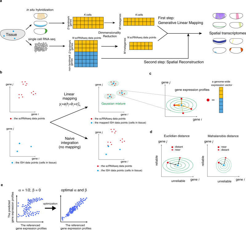
Fig. 1. Schematic illustration of Perler.

a Flow of data processing. b Generative linear mapping from ISH data to the scRNA-seq space. The left and right panels indicate scatter plots in high-dimensional ISH and scRNA-seq spaces. Because ISH data points did not match scRNA-seq data points (naive integration) in the absence of mapping, ISH data points were mapped in order to fit the scRNA-seq data points the best using the EM algorithm. Blue points indicate ISH data points, red points indicate scRNA-seq data points, and green lines indicate contours of the estimated multivariate Gaussian distribution (see “Methods”). c Reconstruction/prediction of gene expression by Mahalanobis’ metric-based weighting (see “Methods”). Orange arrows indicate weights between scRNA-seq data points to cell k, and their widths reflect the Mahalanobis’ metric-based weights. d Schematic demonstrating the difference between Euclidian and Mahalanobis distance. The expression levels of gene i are not reliable as this gene has high noise intensity, while gene j has low noise intensity, thus, its expression levels are considered reliable. In the Mahalanobis distance, the expression levels of each gene are considered by a variance scale. Note, although the “star” scRNA-seq data point is nearer to the ISH data point than the “circle” scRNA-seq data point in Euclidian distance, the weight of the “‘star” data point is smaller than that of the “circle” point. e Weight determination. The hyperparameters of the weighting function, α and β, are determined by cross-validation to ensure that the referenced gene-expression profiles correlate well with the predicted gene-expression profiles (see “Methods”). Dots correspond to cells in tissue. The left and right panels indicate the conceptual scatter plots of the expression levels of the genes before (α = 1/2, β = 0) and after parameter optimization, respectively.