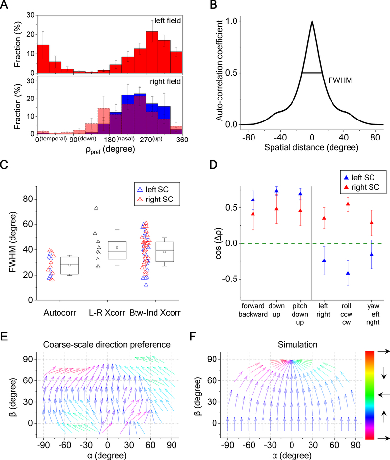
Figure 7. Bias at Various Scales in the Direction Map.

(A) Distribution of preferred directions encountered in both visual hemifields (9 animals). Error bars represent one standard error across animals. Bottom: The histogram for the left hemifield was flipped about the vertical and overlaid on the histogram for the right hemifield.

(B) The radial profile of autocorrelation for a sample direction map. Full-width at half maximum (FWHM) is indicated.

(C) Box plots of the FWHM for the autocorrelation, the cross-correlation between left and right SCs, and the cross-correlation between individuals for the same side of the SC (9 animals). The box plots 25^th to 75^th percentiles, the band inside the box is the median, and the square inside the box is the mean. The ends of the whisker indicate one standard deviation above and below the mean.

(D) Projections of preferred-direction maps from experimental data onto motion maps representing different optic flows (9 animals). Error bars represent one standard error. Wilcoxon signed-rank test or one-sample t-test were applied to test the significance of the difference from 0; the p-values are 4.3e-4, 5.1e-7, 5.0e-6, 0.17, 0.019, and 0.37 for the left SC; 0.098, 0.039, 0.027, 0.019, 1.5e-4, and 0.08 for the right SC. Mann-Whitney U-test or two-sample t-test were applied to test the significance of the difference between left and right SCs, and the p-values are 9.1e-3, 2.5e-5, and 0.061 for the right half figure.

(E) Arrow plots of the preferred direction in the SC, averaged over 9 animals, and plotted across the visual field in unipolar coordinates.

(F) The motion vectors in the mouse’s visual field produced by an aerial predator approaching at constant height from various directions.

See also Figure S7.