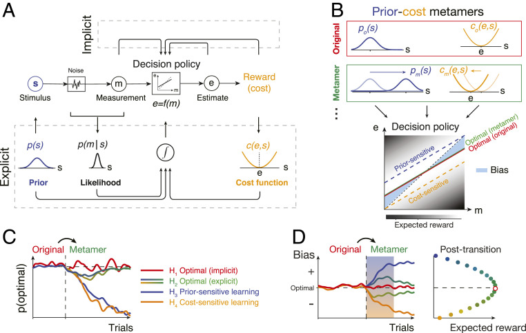
Fig. 1.

Testing Bayesian models of behavior using prior–cost metamers. (A) Ideal-observer model. An agent generates an optimal estimate (e) of stimulus (s) based on a noisy measurement (m). To do so, the agent must compute the optimal decision policy (rectangular box; e = f(m)) that maximizes expected reward. The decision policy can be computed using either an implicit (Top) or explicit (Bottom) learning strategy. In implicit learning, the policy is optimized through trial and error (e.g., model-free reinforcement learning) based on measurements and decision outcomes (arrows on top). In explicit learning, the agent derives the optimal policy by forming internal models for the stimulus prior probability, p(s), the likelihood of the stimulus after measurement, p(m|s), and the underlying cost function, c(e,s). (B) Prior–cost metamers are different p(s) and c(e,s) pairs that lead to the same decision policy. Red box: an original pair (subscript o) showing a Gaussian prior, p_o(s), and a quadratic cost function, c_o(e,s). Green box: a metameric pair (subscript m) whose Gaussian prior, p_m(s), and quadratic cost function, c_m(e,s), are suitably shifted to the right and left, respectively. (Bottom) The optimal decision policy (e = f(m)) associated with both the original (red) and metamer (green) conditions is shown as a line whose slope is less than the unity line (black dashed line; unbiased). The colored dashed lines show suboptimal policies associated with an agent that is only sensitive to the change in prior (blue) or only sensitive to the change in the cost function (orange). The policy is overlaid on a gray scale map that shows expected reward for various mappings of m to e. (C) Simulation of different learning models that undergo an uncued transition (vertical dashed line) from the original pair to its metamer. H₁ (implicit): after the transition, the agent continues to use the optimal policy associated with the original condition. Since this is also the optimal policy for the metamer, probability of behavior being optimal (SI Appendix, Eq. S16), p(optimal), does not change. H₂ (explicit): immediately after the transition, the agent has to update its internal model for the new prior and cost function. This relearning phase causes a transient deviation from the optimality (blue-to-green and yellow-to-green lines after the switch). After learning, the behavior becomes optimal since the optimal policy for the metamer is the same as the original. H₃ (prior sensitive): the agent only learns the new prior, which leads to a suboptimal behavior. H₄ (cost sensitive): same as H₃ for an agent that only learns the new cost function. (D) Same as C for the response biases as a behavioral metric. Similar to p(optimal) in C, bias of the implicit model (H₁) remains at the optimal level and expected reward remains at the maximum level (Right). The explicit model (H₂) shows transient deviation from the optimal bias (blue-to-green and yellow-to-green lines) and expected reward decreases (Right). Prior-sensitive and cost-sensitive models have opposite signs of biases and larger decrease in expected reward (Right).