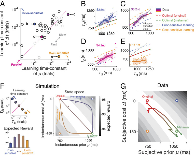
Fig. 5.
Parallel learning of prior and cost function and its computational consequences. (A) Learning time constant for adjusting the mean of the prior (μ) and the shift in the cost function (∆t) after prior–cost transitions. We inferred the learning time constants by fitting exponential curves to learning dynamics (Fig. 4). For many participants, the learning time constants were comparable as evident by the points near the unity line (“parallel,” magenta dotted line). Points above the unity line indicate faster adjustment for μ relative to ∆t, which is expected from a participant that is more prior sensitive (blue circle). Points below the unity line indicate faster adjustment for ∆t relative to μ, which is expected from a participant that is more cost sensitive (orange circle). Two outlier data points on the Top Right were not included in the plot (n = 40 across subjects and sessions). (B–E) Behavior of four example participants in the first 45 posttransition trials (dots: individual trials; solid line: average across bins; shaded region: SEM). The title of each plot indicates the participant (e.g., S2) as well as the session with transitions (e.g., “second”), and the colors correspond to the specific points in A. For each example, the predictions from various optimal and suboptimal models are also shown (legend). (F) Simulation with varying learning time constants. (Top Left) We selected five pairs of the learning time constants for μ and ∆t, indexed by the corresponding time constants, τ, and τΔt, respectively. The pairs ranged from faster prior learning (blue), to parallel learning (brown), to faster cost learning (orange). (Right) Learning trajectory of μ and ∆t for three example points in the Top Left (with the corresponding colors) during the transition from the original prior–cost set (red circle) to its metamer (green circle). Faster prior learning first moves the state toward the prior-sensitive model (open blue circle) and then toward the end point. Faster cost learning first moves the state toward the cost-sensitive model (open orange circle). When the learning time constants are identical (brown), the state moves directly from the original to the metamer. The gray scale color map shows expected reward as a function of μ and ∆t (SI Appendix, Eq. S19). (Bottom Left) Average reward along the learning trajectory for the points in the Top Left. Results correspond to the averages of 500 simulated trials (error bar: SEM). (G) Learning trajectories across participants based on average learning time constants in A shown separately while transitioning from original to metamer (red to green) and from metamer to original (green to red). Note that, on average, the expected reward (gray scale color map, same as F) remains high.

