Pix2pix Conditional Generative Adversarial Networks for Scheimpflug Camera Color-Coded Corneal Tomography Image Generation

Abstract

Purpose

To assess the ability of pix2pix conditional generative adversarial network (pix2pix cGAN) to create plausible synthesized Scheimpflug camera color-coded corneal tomography images based upon a modest-sized original dataset to be used for image augmentation during training a deep convolutional neural network (DCNN) for classification of keratoconus and normal corneal images.

Methods

Original images of 1778 eyes of 923 nonconsecutive patients with or without keratoconus were retrospectively analyzed. Images were labeled and preprocessed for use in training the proposed pix2pix cGAN. The best quality synthesized images were selected based on the Fréchet inception distance score, and their quality was studied by calculating the mean square error, structural similarity index, and the peak signal-to-noise ratio. We used original, traditionally augmented original and synthesized images to train a DCNN for image classification and compared classification performance metrics.

Results

The pix2pix cGAN synthesized images showed plausible subjectively and objectively assessed quality. Training the DCNN with a combination of real and synthesized images allowed better classification performance compared with training using original images only or with traditional augmentation.

Conclusions

Using the pix2pix cGAN to synthesize corneal tomography images can overcome issues related to small datasets and class imbalance when training computer-aided diagnostic models.

Translational Relevance

Pix2pix cGAN can provide an unlimited supply of plausible synthetic Scheimpflug camera color-coded corneal tomography images at levels useful for experimental and clinical applications.

Introduction

Computer-aided diagnosis (CAD) systems could potentially complement medical image interpretation and augment image representativeness and classification, reducing workload, and improving diagnostic accuracy in medical examinations,^1–4 but require large amounts of data for model training. Annotated training data are scarce and costly to obtain. The widespread availability of such data may facilitate the development and validation of more sophisticated computational techniques, overcoming issues of imbalanced datasets and patient privacy concerns.^5–8 Traditional image augmentation techniques are commonly performed to prevent class imbalance in datasets. These techniques include various image transformations, such as rotation, translation, channel splitting, etc. Alternatively, generative adversarial network (GAN), due to its proven ability to synthesize convincingly realistic images, has been used for image augmentation.^7–13

GANs are neural network models in which a generation network and a discrimination network are trained simultaneously. Integrated network performance effectively generates new plausible image samples that are useful for counteracting the domain shift.⁹ Unconditional synthesis refers to image generation without any other conditional information, in which the generator uses random noise as input and outputs synthetic data samples.¹⁰ However, if auxiliary conditional information (most commonly an image) is provided during the generation process, the GAN can be driven to output images with desired properties. A GAN, in this case, is usually referred to as a conditional GAN (cGAN).¹¹ Isola et al. introduced the pix2pix cGAN framework as a general solution to supervised image-to-image translation problems.¹² Its generator receives an image from the input domain and translates it to the target domain by minimizing the pixel-reconstruction error, as well as the adversarial loss, fed back from the discriminator. The discriminator is also tasked with differentiating between the fake output of the generator and the desired ground-truth output image until reaching an equilibrium with the generator.¹³ Keratoconus, a corneal ectatic disorder, is characterized by progressive corneal thinning, causing corneal protrusion, irregular astigmatism, and decreased vision.¹⁴ The best current and widely available diagnostic test to diagnose early keratoconus is tomography (Scheimpflug or corneal coherence tomography). These devices can measure both anterior and posterior corneal surfaces, produce a corneal thickness map, and reconstruct the anterior surface.¹⁵ The Pentacam rotating Scheimpflug camera (Oculus, Wetzlar, Germany) can provide optical cross-sectioning tomography that displays corneal measurement indices in a color-coded fashion: green, yellow, and light blue indicate near-normal values, and red and purple indicate the need for caution, typically in the form of refractive 4-map displays.¹⁶ Several studies have proven the sensitivity and specificity of keratoconus detection using machine learning.^2–4,17,18 Recently, deep learning based on the whole image of corneal color-coded maps obtained with a Scheimpflug camera was used for accurate discrimination between normal and keratoconic eyes.¹⁹ This emerging research field may benefit greatly from medical image synthesis, which can affordably provide an arbitrary number of sufficiently diverse synthetic images that mimic the real Pentacam images. This would permit successful training of a deep-learning network by mitigating the intrinsic imbalance in real imaging datasets, which contain relatively fewer keratoconus and subclinical keratoconus images than normal images. Nevertheless, the pix2pix cGAN has not been used in this context to date.

We assessed the efficacy of a cGAN implementing pix2pix image translation for image synthesis of color-coded Pentacam 4-map refractive displays of clinical and early keratoconus as well as normal corneas. The quality of the synthesized images was attested subjectively and objectively across the different generated image classes. The additive value of the synthetic datasets to manage the shortage of original keratoconus images was assessed by monitoring the classification performance, of a DCNN after training using synthetic, original images with or without traditional image augmentation techniques or combinations of both. We also provided a plausible conventional annotated version of the synthesized images for added value in clinical applications.

Patients and Methods

Study Population

This study followed the tenets of the Declaration of Helsinki, in compliance with applicable national and local ethics requirements. The institutional review board of Assiut University Hospital approved this single-center retrospective analysis and waived the need for patient consent. High-quality corneal Pentacam Scheimpflug (Pentacam HR, Oculus Optikgeräte GmbH, software V.1.15r4 n7) images of 1778 eyes of 923 nonconsecutive, refractive surgery candidates, and patients with unilateral or bilateral keratoconus, obtained between July 2014 and March 2019, were independently analyzed by two experienced corneal specialists (H.A. and K.A; 8 years’ experience). Facilitated by anonymized clinical examination charts, the anonymized images were classified into keratoconus (K), early keratoconus (E), and normal (N) groups, using the following criteria: keratoconus group (K), those with a clinical diagnosis of keratoconus such as a) the presence of a central protrusion of the cornea with Fleicher ring, Vogt striae, or both by slitlamp examination or b) an irregular cornea determined by distorted keratometry mires and distortion of retinoscopic red reflex or both. In addition, the K group includedthe following topographic findings as summarized by Pińero and colleagues:²⁰ focal steepening located in a zone of protrusion surrounded by concentrically decreasing power zones, focal areas with diopteric (D) values > 47.0 D, inferior-superior (I-S) asymmetry measured to be > 1.4D, or angling of the hemimeridians in an asymmetric or broken bowtie pattern with skewing of the steepest radial axis (SRAX). Early keratoconus group (E) was defined as subtle corneal tomographic changes as the aforementioned keratoconus abnormalities in the absence of slit- lamp or visual acuity changes typical of keratoconus. Normal group (N) comprised refractive surgery candidates and subjects applying for a contact lens fitting with a refractive error of less than 8.0 D sphere with less than 3.0 D of astigmatism and without clinical, topographic, or tomographic signs of keratoconus or early keratoconus. After classification, the labeled images were then reviewed by a third party (A.A.), who identified images with conflicting labels and adjudicated their classes by consensus.

Image Dataset Preprocessing Pipeline

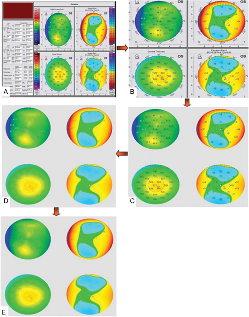
The original dataset comprised 1778 Pentacam 4-maps of refractive display images. Three-hundred-and-four images were classified as clinical keratoconus (K), 584 images as early keratoconus (E), and 890 images as normal (N). All image preprocessing was performed using Python imaging library. All images were cropped, keeping only a square composite image showing the 4-maps without the color-scale bars. Then, images were scaled to 512 × 512 pixels and saved. To remove the background outside the 4-maps, the images were pasted over a gray 512 × 512 background with an intervening third parameter black mask image containing white circles overlapping the four circles of the 4-map display image, to present the 4-maps over a homogenous gray background. All images were then denoised to remove numeric and spatial landmark overlays, leaving only the color codes by iterating over black then white pixel values consecutively replacing the thresholded pixel values with the average value of the nearest neighboring pixels using a Python script. This obviated the use of conventional filters that produce a blurry image with loss of information. At this stage, we isolated a set of randomly chosen 90 images representing each class equally (30 images from each class) to be used as the test set for the classification DCNN. The remaining images (original training set) were used for class-wise training of the pix2pix cGAN and further training/validation of the classification DCNN. Figure 1 depicts image preprocessing steps.

Figure 1.

Image preprocessing pipeline: A) anonymized raw image. B) cropped image. C) background cleanup. D) denoising black maps overlay. E) denoising white maps overlay.

Image Synthesis

Pix2pix cGAN Architecture

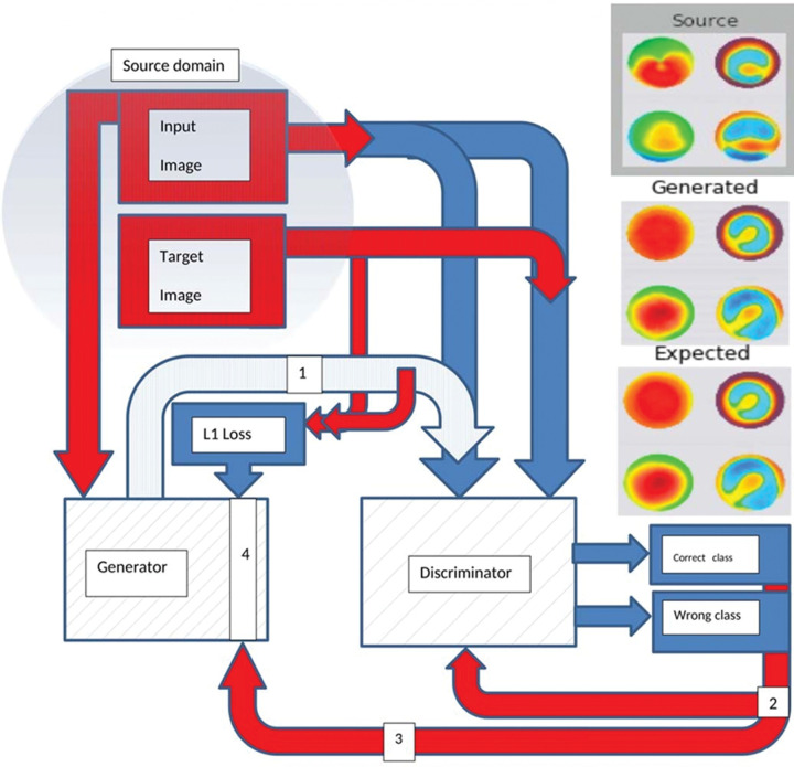
Pix2pix is a type of cGAN, where the generation of the output image is conditional to an input (source) image. The network is made up of two main pieces, the Generator, and the Discriminator. The generator transforms the input image to get the output image. The discriminator measure the similarity of the input image to an unknown image (either a target image from the dataset or an output image from the generator) and tries to guess if this was produced by the generator. The generator is updated to minimize the loss predicted by the discriminator for the generated images.¹¹ To deal with overfitting, the generator is never shown the training dataset clearly, instead dropout layers used during both training and prediction act as the source of randomness with the generator guided by the loss functions throughout training progress.¹³

The Generator

The generator is an encoder-decoder model using a U-Net architecture²¹ The model takes a source image and generates a target image. It does this by first downsampling or encoding the input image down to the bottleneck layer, then upsampling or decoding the bottleneck representation to the size of the output image. The U-Net architecture does not have any fully connected layers, which are replaced by upsampling operators with added skip connections between each convolutional layer.

The Discriminator

The discriminator network design is based on the effective receptive field of the model, which defines the relationship between one output of the model to the number of pixels in the input image. This is called a PachGAN architecture that maps each output prediction of the model to a 70 × 70 square patch of the input image (the patches overlap a lot since the input images are 512 × 512). The benefit of this approach is that the same model can be applied to input images of different sizes, for example, larger or smaller than 512 × 512 pixels.

Loss Function

The discriminator model can be updated directly, whereas the generator model must be updated via the discriminator model. This can be achieved by defining a new composite model that uses the output of the generator model as input to the discriminator model. This composite model involves stacking the generator on top of the discriminator. The generator is updated to minimize the loss predicted by the discriminator for the generated images marked as “original.” As such, it is encouraged to generate more realistic images. The generator is also updated to minimize L1 loss or mean absolute error between the generated image and the target image. This is accomplished by using the weighted sum of both the adversarial loss from the discriminator output and the L1 loss (100 to 1 in favor of L1 loss) to update the generator. This weighing encourages the generator strongly towards generating more realistic translations of input images in the target domain. We implemented the model architecture and configuration proposed by Isola et al.,¹² with minor modifications needed to generate color images of 512 × 512 pixels using Keras 2.3.1 and Tensorflow 2.0.0 libraries.^21,22 The proposed model architecture is illustrated in Figure 2.

Figure 2.

A simplified plot of the proposed composite pix2pix model outlining its main components and workflow (created by Hazem Abdelmotaal). 1: generated image. 2: discriminator loss (D = 0.5 × discriminator cross-entropy loss). 3: adversarial loss. 4: composite loss function (generator loss = adversarial loss + lambda (10) × L1 loss). L1 loss = mean absolute error between the generated image and the target image.

Pix2pix cGAN Training

Three identical pix2pix cGAN models were trained using all available images of each class (after excluding the test set as described). The preprocessed images of each class were loaded as randomly paired images for the source and corresponding target images. The loaded image pairs are scaled so that all pixel values are between −1, +1 instead of 0, 255. Typically, GAN models do not converge, instead, an equilibrium is found between the generator and discriminator.²³ Thus, we cannot easily judge when training should stop. Therefore, we saved the model with its weights regularly during training iterations to be used to generate sample images for quality assessment. This allowed selecting the best model weights that allow for generating the best quality images. Model weights were initialized via random Gaussian with a mean of 0.0 and a standard deviation of 0.02. Adam (Adaptive moment estimation) optimizer version of stochastic gradient descent²⁴ with a small learning rate of 0.0002 and modest momentum (first momentum term (β₁) = 0.5 and second momentum term (β₂) = 0.999). As the training of the discriminator is too fast compared to the generator, the loss for the discriminator is weighted by 50% for each model update to slowdown the discriminator training (discriminator loss = 0.5 × discriminator loss). The number of training iterations (epochs) was set at 200 with a batch size of 1. The generator was saved every 10 epochs. Consequently, we obtained 20 saved generator model files with their weights.

Selection of Synthesized Images With the Best Quality

As training progresses the generated image quality is expected to improve, however, more training epochs does not necessarily mean better quality images. In fact, image quality may fall by further training after reaching optimum quality in earlier epochs. So, a final generator model can be chosen based on generated image quality, not total training epochs. Therefore, we can choose a model based on the quality of the generated images. This can be accomplished by loading each model and making ad hoc translation of source images in the training dataset for subjective or objective assessment.⁵

To select the generator epoch that produced the best image quality, we used the Fréchet inception distance (FID) score,²³ which is a metric that calculates the distance between feature vectors calculated for original and generated images. The score is calculated using the Inception V3 model used for image classification. It specifically uses the coding layer of the model (the last pooling layer before the output classification of images) to capture computer-vision-specific features of an input image. These activations are calculated for a collection of original and generated images. The activations are summarized as multivariate Gaussian by calculating the mean and covariance of the images. These statistics are then calculated for the activations across the collection of original and generated images. The distances between these two distributions are then calculated using the Fréchet distance, also called the Wasserstein- 2 distance. A higher score indicates lower quality images, conversely, a lower score indicates that the two groups of images are more similar, and the relationship may be linear. A perfect score of 0.0 indicates that the two groups of images are identical.

We used the FID score to select the best generator epoch for each image class to avoid bias introduced by subjective evaluation. Also, differences in image quality produced by the generator during successive training epochs may be undetectable by the human eye, even with experienced observers. The best model generators with weights that produced the best synthesized image quality per class were employed for image synthesis, and the synthesized image quality was evaluated subjectively and objectively.

Subjective Visual Quality Evaluation

One hundred and fifty synthesized images representing each image group equally were visually evaluated for global consistency and image content by the same experienced corneal specialists (H.A. and K.A.) who classified the original dataset. They subjectively evaluated the overall quality of images on a scale of 1 to 5 (1 = excellent, 2 = good, 3 = normal, 4 = poor, and 5 = very poor). The quality of the original images was used as the standard for score 1.

Objective Evaluation Metrics for Synthesized Images

To objectively assess the synthesized image quality, all per-class images obtained from the selected model generators were quantitatively evaluated using the mean square error (MSE), structural similarity (SSIM) index, and the peak signal-to-noise ratio (PSNR).^25–27 The MSE represents the cumulative squared error between the synthesized and original images. The SSIM index measures the structural information similarity between images, where 0 indicates no similarity and 1 indicates complete similarity. The PSNR measures image distortion and noise level between images; a higher PSNR value indicates higher image quality.⁵

Evaluation of Classification Performance

Deep neural networks trained with a combination of real and synthesized images have a potential advantage over networks trained with real images alone, including a larger quantity of data, better-diversified datasets, and preventing overfitting.

Classification Network Structure

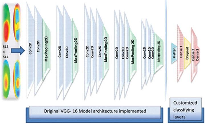
To gauge the performance gains obtained by employing pix2pix cGAN-based image augmentation, we benchmarked the images synthesized by the employed algorithm using the VGG-16 network. The VGG-16 (also called OxfordNet) is a convolutional neural network that is 16 layers deep named after the Visual Geometry Group from Oxford, who developed it. It was used to win the ImageNet Large Scale Visual Recognition (iLSVR) Challenge in 2014.²⁸ The VGG-16 is widely employed in several medical image classification tasks. The pretrained VGG-16 DCNN with ImageNet weights was used and customized for image classification. After modifying the input tensor shape of the top dense layer, thereby forcing the model to accept the shape 512 × 512 of the input images, the last classifying layers of the model were truncated and replaced by a flattened layer followed by two fully connected layers (64 nodes- dense 1 and 2) separated by a dropout layer and followed by a final fully connected (3 nodes- dense 3) layer with softmax activation adapted to output the three image classes. The model architecture is shown in Figure 3. The model was initialized with ImageNet weights. Model hyperparameters were fine-tuned manually searching for the best values of momentum, dropout rate, and learning rate that fit with various input data instances. This entailed using a first momentum term (β₁) between 0.9 and 0.6 with the default second momentum term (β₂) = 0.999. The learning rate was reduced by a factor of 0.2 when validation loss stops improving for three epochs with a lower bound of learning rate = 0.001 to prevent increasing loss at high learning rates with a subsequent drop in accuracy. The dropout rate used ranged between 0.1 and 0.3.

Figure 3.

The proposed custom VGG-16 model architecture used for 512 × 512 pixel image classification (created by Hazem Abdelmotaal). Conv2D = convolution layer + ReLU activation; Dense 1, 2 = fully connected layers + ReLU activation; Dense 3 = fully connected layer + Softmax activation.

Training Datasets

We trained the aforementioned classifier using six different combinations of the original training set and synthesized 4-map refractive display images (Fig. 4).

• 1.Balanced original dataset (BO): A balanced version of the original training image samples, where the number of 4-map refractive display image samples per class was set to the maximum number of available original training image samples in the least represented class (K).
• 2.Imbalanced original dataset (IO): All available original training image samples were used.
• 3.Imbalanced original dataset with traditional augmentation (IOA): All available original training image samples were augmented by artificially increasing their number using traditional image augmentation, by slight rotation, width-shift, height-shift, and scaling, without using vertical or horizontal flip, to avoid unrealistic image deformation.
• 4.Imbalanced original dataset partly augmented with synthesized images (IOPS): A concatenation of all available original training and augmented synthesized images in E and K classes, to enlarge the number of image samples to equal the maximum number of available original training images in the most plentifully represented class (N).
• 5.Imbalanced original dataset fully augmented with synthesized images (IOFS): A concatenation of all available original training and augmented synthesized images in all classes to enlarge the number of image samples per class to twice the maximum number of original training images in class N.
• 6.Balanced synthesized dataset (BS): A balanced version of 3000 synthesized images representing each class (total 9000 images) was used for training without using the original training dataset. As the pix2pix model outputs images with 512 × 512 resolution, no rescaling of synthesized images was needed before combining with original images. During training, we used a 0.3 validation split, which is the fraction of the training data to be used as validation data.²⁹ The model will set apart this fraction of the training data, will not train on it, and will evaluate the loss and any model metrics on this data at the end of each epoch. Class weights were fed to the model, therefore, imposing a cost penalty on the minority class misclassification. These penalties ask the model to pay more attention to minority classes preventing the model from being biased toward the majority class. The number of training iterations (epochs) was set to 10. The model was implemented using Keras 2.3.1 and TensorFlow 2.0.0 libraries.^20,22 Each trained model was used for the classification of the test set only once, and classification metrics were recorded.

Figure 4.

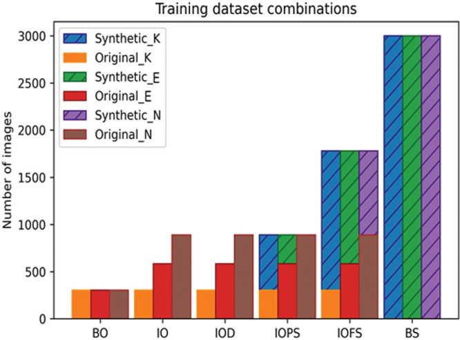
The number of samples per training dataset. BO: balanced original dataset; BS: balanced synthesized dataset; IO: balanced original dataset; IOA: imbalanced original dataset with traditional augmentation; IOFS: Imbalanced original dataset fully augmented with synthesized images; IOPS: imbalanced original dataset partly augmented with synthesized images; E: early keratoconus images; K: keratoconus images; N: normal cornea images.

Performance Metrics

The VGG-16 classifiers’ performance on the test set was analyzed, based on model accuracy, precision, recall, F1 score, and receiver operating characteristic curve (ROC) analysis.³⁰

Synthesized Image Annotations

To obtain synthesized 4-map refractive display images with a realistic appearance, we used an image annotation algorithm for automated input of numerical and landmark overlay using Python imaging library. This essentially sought to reverse changes made during original image preprocessing to yield synthesized images with a realistic appearance that could be used for other research and clinical training purposes. Firstly, the synthesized images were concatenated with a squared background template containing all image features outside the four circles containing the maps. Then the numeric annotations were printed guided by automated matching of the synthesized map pixel values and the values of the relevant color scale at the same conventionally selected points in each map. The corneal pachymetric apex was marked by an opaque white circle, the corneal thinnest location was marked by a transparent black circle, and the maximum curvature power on the front of the cornea (K-Max (front)) was marked by the conventional white opaque vertical rhombus. All these landmarks were also calculated from the synthesized color codes. Landmarks outlining the pupil were fake circles chosen at random diameter between 3 and 6 mm printed in all four maps with a central striped cross indicating the presumed position of the pupil center. One hundred and fifty synthesized annotated images representing each image group equally were randomly chosen and shuffled with an equivalent number of original images and presented to different experienced corneal specialists (A.F. and D.E), and they were asked to classify the images as real and fake. Another class-balanced synthesized annotated dataset comprising 150 images was supplied to the same readers for classification into keratoconus, early keratoconus, and normal classes and inter-rater agreement was estimated. Also, readers were asked to report the overall quality scores of the synthesized annotated images compared to original unprocessed images in the same 1 to 5 score used before.

Statistical Analysis, Computer Hardware, and Software

All statistical analyses were performed using SciPy (scientific computing tools for Python) and scikit-learn (version 0.21.3).³¹ Scikit-learn is a Python module for machine learning built on top of SciPy. Patient data are presented as means and standard deviations. Analysis of variance was used to compare means of image group metrics. The Mann-Whitney U test was used for the analysis of the means of the five-point assessment score given by the two readers, and P < 0.05 was considered significant. Inter-rater agreement was estimated with Cohen's к. Model performance was assessed by estimating precision, recall, F1 score, accuracy, and ROC curve. The one-versus-all approach was applied to extend the use of ROC curves into three classes (each class was taken as a positive class while the other two classes were jointly considered as the negative). Deep-learning computations were performed on a GPU composed of a personal computer with a GeForce RTX 2060 SUPER graphics card powered by an NVIDIA Turing architecture with a CUDA 11.0.126 drive.

Results

Table 1 summarizes the characteristics of the study population. Inter-rater agreement for classification of original dataset was 0.92 (Cohen к 0.86). This trivial ground-truth label noise ensured the presence of robust characteristics that the pix2pix cGAN can use for the class-specific style transfer in the synthesized images. Also, these clear characteristics facilitate feature extraction by the classifier during VGG-16 training.

Table 1.

Characteristics of the Study Population

Parameter	Keratoconus	Early Keratoconus	Normal
Subjects/eyes (n)	158/304	303/584	462/890
Age (y)	29.7 ± 2.2	30.3 ± 2.8	33.3 ± 8.1
Kƒlat (D)	45.95 ± 6.6	43.82 ± 3.8	42.02 ± 2.4
Ksteep (D)	49.28 ± 6.5	45.92 ± 2.6	44.46 ± 1.6
Astigmatism (D)	3.50 ± 3.25	1.50 ± 0.75	1.25 ± 1.50
TCT (µm)	423.45 ± 635.84	495.56 ± 23.80	536.66 ± 44.32
I – S value (D)	4.82 ± 2.86	0.06 ± 0.34	0.96 ± 1.06

I – S value = inferior- superior asymmetry; K _ƒlat = keratometric power in the flattest meridian, K _steep = keratometric power in the steepest meridian; TCT = thinnest corneal thickness. Data are given as mean ± standard deviation.

Dataset Preprocessing

After preprocessing the original image dataset, we obtained 304 class K, 584 class E, and 890 class N images. The process of removing the background annotation noise was not quite successful, with the maps still exhibiting noticeable salt and pepper background noise. However, this noise can act as a source of data augmentation later when these images are used for assessment of VGG-16 classification performance to ensure that the model can learn robust representations. We randomly selected 90 images from the original dataset representing each class equally (30 images per class). These images were set apart to be used as the test set for the classification DCNN. The remaining images (274 class K, 554 class E, 860 class N) were used as the training set for class-wise training of the pix2pix cGAN and further training/validation of the classification DCNN.

Pix2pix cGAN Training and Generator Selection

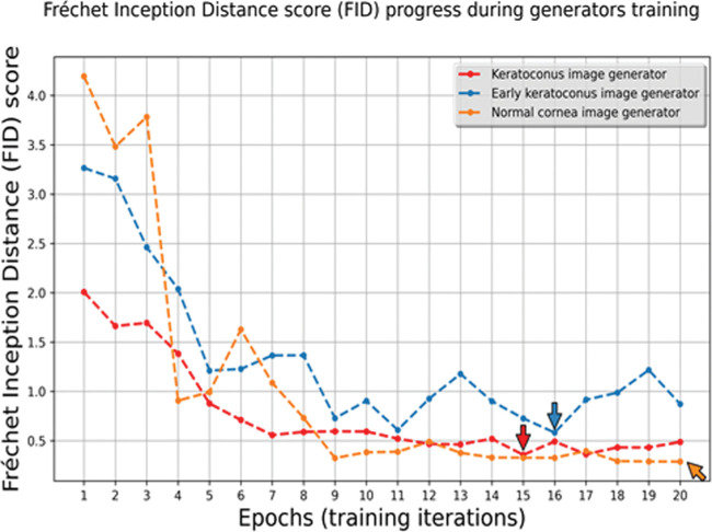
Pix2pix cGAN training for 200 epochs took on average 12 hours for each class. The saved trained generators were used to synthesize image samples. The FID score was calculated for images obtained by each of the 20 saved generators per image class. FID scores tended to improve with training progress (Fig. 5); however, the best FID score was reached at the 15^th epoch for the class K image generator, at the 16^th epoch for the class E image generator, and at the 20^th epoch for the class N image generator. Training of K and E image generators beyond this point produced lower FID scores, highlighting the importance of this metric for defining the best generator epoch for image synthesis. These generators were selected for further per-class image synthesis in the study.

Figure 5.

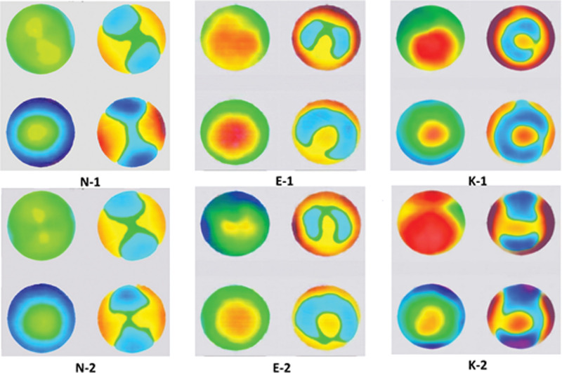
Synthetic image examples. E-1, E-2: early keratoconus images; K-1, K-2: keratoconus images; N-1, N-2: normal cornea images.

Subjective Image Evaluation

Figure 6 shows some samples of synthetically generated images. The images were globally consistent because the model learned to introduce visual content only in the four circular fields of the maps. The color code distribution also shows high plausibility. It is noticeable that the black and white background noise present in the original preprocessed images almost disappeared in the synthesized images meaning that the model could identify these artifacts as irrelevant during learning, effectively excluding them in the synthesized images. Compared with the preprocessed original image in Figure 1, we can see that these generated output images are visually close to real ones. In the five-point assessment of the overall image quality, the mean of the scores given by the first reader was 2.24 ± 0.44, 2.96 ± 0.98, 2.78 ± 0.70, and by the second reader 2.08 ± 0.62, 2.56 ± 0.20, 2.16 ± 0.92 for the K, E, and N classes synthesized images, respectively. This reflects the good quality of synthesized images in all classes. There was no significant difference between classes’ average scores given by both readers (P = 0.0921, P = 0.395, P = 0.477 for K vs. E, K vs. N, and E vs. N, respectively). This reflects that the models generated class-specific features efficiently.

Figure 6.

The Fréchet inception distance (FID) score changes during training. The arrows point to the epochs (training iteration) with the best-generated image FID score per class.

Objective Image Evaluation Metrics

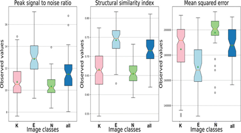
All available original preprocessed training image samples in each class were used for pairwise comparison with an equivalent number of synthesized images of the same class by calculating the PSNR, SSIM, and MSE. As all the quality scores had a normal distribution according to the Kolmogorov‒Smirnov test, data were expressed as mean ± standard deviation (Fig. 7, Table 2). The generated class E images had the least distortion and noise and had the maximum positive similarity to their corresponding original counterparts. However, the PSNR and SSIM metrics did not differ significantly among image classes by one-way ANOVA (F = 36.858, P = 1.06; F = 76.051, P = 4.66, respectively). The average SSIM for all synthesized images was 0.66 ± 0.05, with a maximum value of 0.82, confirming that our model generalized properly and did not trivially memorize the training set samples.

Figure 7.

Box-plot of peak signal-to-noise ratio, structural similarity index, and mean square error between the generated image sample and equivalent sample of all available original images. Images were synthesized by best generator performance according to the best Fréchet inception distance score. The notches in the box-plot represent the confidence interval around the median. The mean is marked by a triangle. E = early keratoconus; K = keratoconus; N = normal cornea.

Table 2.

Characteristics of Generated Image Samples Compared to an Equivalent Sample of All Available Original Images. Images Were Synthesized by Best-Selected Generators, Guided by the Fréchet Inception Distance Score of Their Generated Images.

Image Class	PSNR	SSIM	MSE
Keratoconus	12.87 ± 1.49	0.74 ± 0.04	170771.9 ± 17250.6
Early keratoconus	10.37 ± 1.05	0.66 ± 0.03	197984.3 ± 13525.1
Normal	11.48 ± 1.75	0.71 ± 0.04	187569.6. ± 14085.4
All Classes	10.78 ± .1.45	0.66 ± 0.05	184855.1 ± 20210.4

Note that the standard deviation is calculated as the population standard deviation (PSD), not the sample standard deviation (SSD), representing the total variance rather than the sample image variance.

MSE = mean square error; PSNR = peak signal-to-noise ratio; SSIM = structural similarity index data are given as the mean ± standard deviation.

Classification

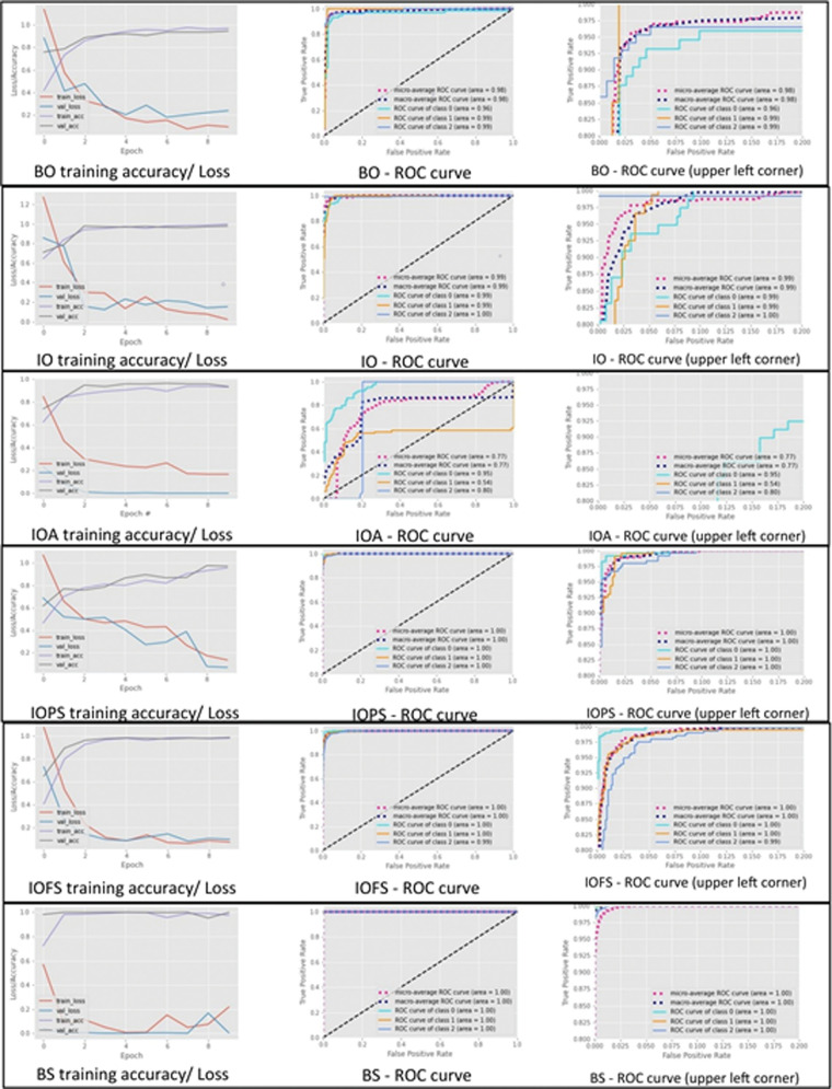
We assessed the performance of the VGG-16 DCNNs trained on six different combinations of original and synthesized images in the classification of the test set. Model accuracy, precision, recall, and F1 score are presented in Table 3. Plots of the corresponding training and validation accuracy/loss scores and ROC curves for the classification of the test set are presented in Figure 8. The use of synthesized images during training increased classification performance, supporting their use for augmenting training sets. Additionally, balancing the training set appeared to have minimal value in improving classifier performance, as compared to the overall increase in the training dataset volume, with the best results obtained by integrating the two techniques. ROC plots showed that adding synthesized images to the training set could improve the trade-off between false-positive and true-positive rates during the classification of the test set. Furthermore, average per-class precision, recall, and F1 score values showed that N images were easier to classify, while differentiation between K and E images was more challenging. F1 scores for class K classification of the test set were reduced when shifting from training using the BO dataset to the IO dataset, despite using the same number of original class K images during training, mostly due to lower recall and reflecting the impact of class imbalance. Traditional augmentation performed worst, with the model failing to identify E images better than random guessing, highlighting the limited usefulness of traditional augmentation techniques for color-coded images with precise spatial structural content. The model trained solely on 9000 synthesized image datasets outperformed the models fed by other, less-plentiful image combinations. Additionally, model overfitting during training/validation was observed with relatively smaller training dataset domains and was the main cause of the need for hyperparameter fine-tuning during training phases.

Table 3.

Classification Accuracy, Precision, Recall, and F1 score of VGG-16 Model, for the Test Dataset After Training Using Each Image Combination. Results Are Shown After Normalization

Training Dataset	Image Class	Precision	Recall	F1-Score	Accuracy (%)
	Keratoconus	0.93	1.0	0.96
BO	Early keratoconus	1.0	0.92	0.96	97.33
	Normal	1.0	1.0	1.0
	Keratoconus	0.93	0.84	0.88
IO	Early keratoconus	0.92	0.97	0.94	95.87
	Normal	1.0	0.99	0.99
	Keratoconus	0.97	0.42	0.58
IOA	Early keratoconus	0.49	0.57	0.53	64.89
	Normal	0.68	1.0	0.81
	Keratoconus	0.99	0.98	0.98
IOPS	Early keratoconus	0.98	0.99	0.99	98.67
	Normal	0.99	1.0	0.99
	Keratoconus	0.99	1.0	0.99
IOFS	Early keratoconus	0.99	0.99	0.99	99.56
	Normal	1.0	1.0	1.0
	Keratoconus	1.0	0.99	1.0
BS	Early keratoconus	0.99	1.0	1.0	99.78
	Normal	1.0	1.0	1.0

BO: balanced original dataset; BS: balanced synthesized dataset; IO: unbalanced original dataset; IOA: imbalanced original dataset with traditional augmentation; IOFS: unbalanced original dataset fully augmented with synthesized images; IOPS: unbalanced original dataset partially augmented with synthesized images.

Figure 8.

Plots of receiver operating characteristic (ROC) curves for test set classification and the corresponding accuracy/loss scores during the training/validation process by each dataset combination. During training, the accuracy increases, while the loss, representing the error, decreases. The one-versus-all approach was applied to extend ROC curve use in this 3-class problem, in which each class is considered a positive class while the other two classes are jointly considered as the negative class. Class 0 = keratoconus, class 1 = normal, class 2 = early keratoconus. The right-side plots are close-up views of the upper left corner of the graph. BO: balanced original dataset; BS: balanced synthesized dataset; IO: imbalanced original dataset; IOA: imbalanced original dataset with traditional augmentation; IOFS: imbalanced original dataset fully augmented with synthesized images; IOPS: imbalanced original dataset partly augmented with synthesized images. Micro-average ROC curve = the precision (true positives [TP] / TP + false positives [FP]) from the individual TP and FP of each class (precision-micro = TP0 + TP1 + TP2 / TP0 + TP1 + TP2 + FP0 + FP1 + FP2). Macro-average ROC curve = the average precision of the three classes (precision-macro = (precision 0 + precision 1 + precision 2)/3).

Automated Annotation Algorithm

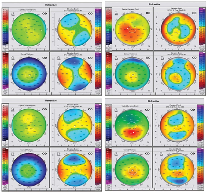
The generated images were copied, and an automated annotation algorithm was used to give them a conventional, clinically useful appearance. Figure 9 shows some randomly selected samples of synthetically generated images after annotation. Numerical values and positions of markings are plausible and can aid human classification performance. Inter-rater agreement for original/synthetic image discrimination was 0.42 (Cohen к 0.18), indicating slight inter-rater agreement; this implies that the original and synthesized annotated copies are fairly similar. Inter-rater agreement for classification of the synthesized dataset was 0.90 (Cohen к 0.84); this implies that the synthetic images contained robust characteristic features allowing for accurate classification by human readers. In the five-point assessment of the overall synthetic image annotation quality, the mean of the scores given by the first reader was 1.74 ± 0.55, 2.22 ± 0.12, 2.00 ± 0.64, and for the second reader 2.28 ± 0.94, 3.16 ± 0.20, 2.50 ± 0.80 for the K, E, and N synthesized images classes, respectively. This reflects the good quality of the annotation algorithm.

Figure 9.

Examples of annotated synthetic images.

Discussion

The present study showed that applying the pix2pix cGAN to color-coded Scheimpflug corneal maps can efficiently generate images with plausible quality in N, K, and E classes. To date, no previous study has reported the use of the pix2pix cGAN in this type of image translation task. The basic pix2pix framework has been used for medical image denoising, reconstruction, or segmentation, rather than for amplifying the original dataset.^32,33 Although the background annotation noise can easily be avoided by exporting Pentacam data from the beginning, rather than using screenshots, we preferred to utilize the more commonly used conventional annotated images to facilitate retrospective studies of stored images by interested researchers and allow comparison between ground-truth annotated images and their synthesized annotated counterparts. Fujioka et al. demonstrated that, with increasing epoch number, the final image quality increased. However, they postulated that overlearning may occur if learning extended beyond the ideal number of learning iterations.³⁴ Previous studies used subjective scores by experienced raters to select generator epochs producing the best image quality.^6–8,35 However, this method may introduce bias, due to inter- and intraindividual rater variations. We used the newly developed FID score as an objective metric to gauge the generated image quality after each learning iteration, instead of relying on human observers. We confirmed that continuing learning beyond the optimal epoch can result in a lower-quality image-generating performance. Our method could provide synthetic Pentacam corneal tomography images with plausible subjective and objective qualities in keratoconus, early keratoconus, and normal cornea domains, comparable to other studies implementing pix2pix networks for other image datasets.^5,6 Yu et al. documented better PSNR and SSIM when using the pix2pix framework than the CycleGAN.^5,36 We also postulate that unpaired training with the CycleGAN does not have a data fidelity-loss term; therefore, preservation of small abnormal regions during the translation process is not guaranteed. Rozema et al.³⁷ used a stochastic eye model to generate realistic random Gaussian distortions, which were superimposed on the anterior corneal surface to simulate statistical and epidemiological properties of keratoconus. Their model was capable of generating an unlimited number of keratoconus biometry sets. However, parameter reduction in their model comes at the expense of information loss which reduces parameter variability. This modeling is different from our approach, which maps high-dimensional images into a latent space where high-level features are extracted from individual pixels. This latent space is used to morph original images into new analogous images under constraints imposed by the loss functions and the source image domain. This permits unlimited synthesis of convincingly realistic and phenotypically diverse images that retain high-level feature similarity. In DCNNs, there is always a trade-off between the training dataset size, model complexity, nature of the data, and performance.⁷ Our results showed that increasing the training dataset size with synthesized images resulted in robust classification performance and decreased model overfitting, improving the network's generalizability to unseen test data, consistent with other studies using different datasets.⁷ In our dataset, traditional augmentation resulted in poor classifier performance, possibly due to the introduction of inconvenient spatial variance, which may prevent the classifier from identifying the most influential image pixels, resulting in model underfitting. This was inconsistent with the findings of other studies^7,19,38 using different datasets and more training iterations and hyperparameter modulation. Another perspective could be that with traditional augmentation strategies, the abnormality classifier may find it relatively difficult to approximate the noise function in augmented images as compared to approximating the image features generated by GAN. In this respect, GANs provided a more generic solution. However, as we used a limited number of training iterations with no remarkable changes to the model architecture, further analysis is required to interpret the performance of the VGG-16 classifier, which was beyond the scope of our research. We demonstrated the model overfitting to the smaller training datasets and the limited value of implementing class weights during training to counteract the class imbalance. These findings strongly support the usefulness of the pix2pix cGAN for data augmentation, providing instantaneous high-quality synthetic images of the required amount. The overall subjective evaluations of the synthesized images of all image classes were promising. The presence of artifacts may be partially due to the low amount of data and the transposed convolutions used in the decoder part of the generator architecture.³⁹ Subjective assessment of synthesized images was satisfactory in agreement with objective evaluation results and other reports.^7,35 Also, the quality of the automated annotation algorithm was promising, giving the synthesized images a realistic appearance that challenged human readers in discrimination between original and synthesized images. By simulating conventional maps, the annotation helped human graders in the classification of synthesized images successfully. A better annotation algorithm may optimize similarity with original maps in the future. Our study had some limitations. Generative models are always limited by the information contained within the training set, and how it captures the variability of the underlying real-world data distribution. Given that our data for both image generation and classification were sourced from the same institution, it remains an open question as to whether the results reported here can be generalized to data from other institutions, which may have different population statistics. Additionally, the drawback of the FID score is that the ground-truth samples are not directly compared to the synthetic samples. The score indirectly evaluates synthetic images based on the statistics of a collection of synthetic images compared to the statistics of a collection of real images from the target domain. The absolute VGG-16 classifier performance could potentially be improved by additional architecture and hyperparameter searches, but we focused on assessing classification metrics trends rather than optimizing end performance in this study. Finally, the reliability of synthetic images may be improved by collecting data from more cases.

Conclusions

We demonstrated that the proposed pix2pix cGAN framework trained by using a small size of prospectively labeled color-coded Scheimpflug camera corneal tomography images shows promise in the generation of plausible keratoconus, early keratoconus, and normal 4-map display corneal tomography images at levels that could provide value in many experimental and clinical contexts. The performance and fidelity of the results were positively attested subjectively and objectively across the different generated image classes. Such a network could be a valuable aid to provide synthetic datasets to manage the shortage of labeled data and correct image class imbalance, resulting in substantial improvement in classification performance, while preserving patient privacy and confidentiality. These findings are of paramount importance in respect to training recent DCNNs with deeper architecture and a large number of parameters that may suffer from lack of generalization in training with smaller datasets. Interestingly, we also provided a plausible conventional annotated version of the synthesized images that may provide additive practical value to the synthesized dataset. The natural extension of our work is to construct more customized models to improve the quality of generated images and study their contained semantic structure to better understand the transition pathways between image classes.

References

- 1. Issarti I, Consejo A, Jiménez-García M, Hershko S, Koppen C, Rozema JJ.. Computer aided diagnosis for suspect keratoconus detection. Comput Biol Med. 2019; 109: 33−42. [DOI] [PubMed] [Google Scholar]
- 2. Smadja D, Touboul D, Cohen A, et al.. Detection of subclinical keratoconus using an automated decision tree classification. Am J Ophthalmol. 2013; 156: 237−246. [DOI] [PubMed] [Google Scholar]
- 3. Arbelaez MC, Versaci F, Vestri G, Barboni P, Savini G.. Use of a support vector machine for keratoconus and subclinical keratoconus detection by topographic and tomographic data. Ophthalmology. 2012; 119: 2231−2238. [DOI] [PubMed] [Google Scholar]
- 4. Souza MB, Medeiros FW, Souza DB, Garcia R, Alves MR.. Evaluation of machine learning classifiers in keratoconus detection from orbscan II examinations. Clinics (Sao Paulo). 2010; 65: 1223−1228. [DOI] [PMC free article] [PubMed] [Google Scholar]
- 5. Yu Z, Xiang Q, Meng J, Kou C, Ren Q, Lu Y.. Retinal image synthesis from multiple-landmarks input with generative adversarial networks. Biomed Eng Online. 2019; 18: 62. [DOI] [PMC free article] [PubMed] [Google Scholar]
- 6. Armanious K, Jiang C, Fischer M, et al.. MedGAN: medical image translation using GANs. Comput Med Imaging Graph. 2020; 79: 101684. [DOI] [PubMed] [Google Scholar]
- 7. Salehinejad H, Colak E, Dowdell T, Barfett J, Valaee S.. Synthesizing chest X-ray pathology for training deep convolutional neural networks. IEEE Trans Med Imaging. 2019; 38: 1197−1206. [DOI] [PubMed] [Google Scholar]
- 8. Costa P, Galdran A, Meyer MI, et al.. End-to-end adversarial retinal image synthesis. IEEE Trans Med Imaging. 2018; 37: 781−791. [DOI] [PubMed] [Google Scholar]
- 9. Goodfellow IJ, Pouget-Abadie J, Mirza M, et al.. Generative adversarial networks. ArXiv. 2014;abs/1406.2661.
- 10. Cronin NJ, Finni T, Seynnes O.. Using deep learning to generate synthetic B-mode musculoskeletal ultrasound images. Comput Methods Programs Biomed. 2020; 196: 105583. [DOI] [PubMed] [Google Scholar]
- 11. Lan L, You L, Zhang Z, et al.. Generative adversarial networks and its applications in biomedical informatics. Front Public Health. 2020; 8: 164. [DOI] [PMC free article] [PubMed] [Google Scholar]
- 12. Isola P, Zhu J-Y, Zhou T, Efros AA.. Image-to-image translation with conditional adversarial networks. Proceedings of the IEEE conference on computer vision and pattern recognition. 2017: 1125−1134.
- 13. Zhao J, Mathieu M, LeCun Y.. Energy-based generative adversarial network. arXiv:160903126. 379.2016.
- 14. Piñero DP, Nieto JC, Lopez-Miguel A.. Characterization of corneal structure in keratoconus. J Cataract Refract Surg. 2012; 38: 2167−2183. [DOI] [PubMed] [Google Scholar]
- 15. Gomes JAP, Tan D, Rapuano CJ, et al.. Global consensus on keratoconus and ectatic diseases, Cornea. 2015; 34(4): 359−369. [DOI] [PubMed] [Google Scholar]
- 16. Medghalchi A, Moghadam RS, Akbari M, et al.. Correlation of corneal elevations measured by Scheimpflug corneal imaging with severity of keratoconus. J Curr Ophthalmol. 2019; 6: 377−381. [DOI] [PMC free article] [PubMed] [Google Scholar]
- 17. Ruiz Hidalgo I, Rozema JJ, Saad A, et al.. Validation of an objective keratoconus detection system implemented in a Scheimpflug tomographer and comparison with other methods. Cornea. 2017; 36(6): 689−695. [DOI] [PubMed] [Google Scholar]
- 18. Ruiz Hidalgo I, Rodriguez P, Rozema JJ, et al.. Evaluation of a machine-learning classifier for keratoconus detection based on Scheimpflug tomography. Cornea. 2016; 35: 827−832. [DOI] [PubMed] [Google Scholar]
- 19. Abdelmotaal H, Mostafa MM, Mostafa ANR, Mohamed AA, Khaled Abdelazeem. Classification of color-coded Scheimpflug camera corneal tomography images using deep learning. Trans Vis Sci Tech. 2020; 9(13): 30, 10.1167/tvst.9.13.30. [DOI] [PMC free article] [PubMed] [Google Scholar]
- 20. Chollet F. keras: GitHub, https://scholar.google.com/scholar?hl=en&as_sdt=0,5&q=Francois+Chollet,keras, 2015.
- 21. Ronneberger O, Fischer P, Brox T.. U-net: convolutional networks for biomedical image segmentation. In: International conference on medical image computing and computer-assisted intervention. Cham: Springer; 2015. [Google Scholar]
- 22. Abadi M, Barham P, Chen J, et al.. Tensorflow: a system for large-scale machine learning. In OSDI, 16(2016): 265–283, https://www.usenix.org/conference/osdi16/technical-sessions/presentation/abadi. [Google Scholar]
- 23. Heusel M, Ramsauer H, Unterthiner T, Nessler B, Hochreiter S.. GANs trained by a two time- scale update rule converge to a local nash equilibrium. In NIPS. 2017;6629–6640, https://arxiv.org/abs/1706.08500.
- 24. Kingma DP, Jimmy LB.. Adam: a method for stochastic optimization. 2014. arXiv:1412.6980v9
- 25. Zhou W, Bovik AC, Sheikh HR, Simoncelli EP.. Image quality assessment: from error visibility to structural similarity. IEEE Trans Image Process. 2004; 13: 600−612. [DOI] [PubMed] [Google Scholar]
- 26. Dar SU, Yurt M, Karacan L, Erdem A, Erdem E, Çukur T.. Image synthesis in multi-contrast MRI with conditional generative adversarial networks. IEEE Trans Med Imaging. 2019; 38: 2375−2388. [DOI] [PubMed] [Google Scholar]
- 27. van Stralen M, Wozny PJ, Zhou Y, Seevinck PR, Loog M.. Contextual loss functions for optimization of convolutional neural networks generating pseudo CTs from MRI. In Medical Imaging 2018: Image Processing, 10.1117/12.2293749. [DOI]
- 28. Russakovsky O, Deng J, Su H, et al.. ImageNet large scale visual recognition challenge. Int J Comput Vis. 2015; 115(3): 211–252 [Google Scholar]
- 29. Kohavi R. A study of cross-validation and bootstrap for accuracy estimation and model selection. In: Proceedings of the Fourteenth International Joint Conference on Artificial Intelligence. San Mateo, CA: Morgan Kaufmann. 1995; 2(12): 1137–1143. [Google Scholar]
- 30. Powers DMW. Evaluation: from precision, recall, and F-measure to ROC, informedness, markedness & correlation. J Mach Learn Technol. 2011; 2: 37−63, https://arxiv.org/abs/2010.16061. [Google Scholar]
- 31. Oliphant TE. Python for scientific computing. Comput Sci Eng. 2007; 9: 10−20. [Google Scholar]
- 32. Wolterink JM, Leiner T, Viergever MA, Išgum I.. Generative adversarial networks for noise reduction in low-dose CT. IEEE Trans Med Imaging. 2017; 36: 2536−2545. [DOI] [PubMed] [Google Scholar]
- 33. Chen Y, Shi F, Christodoulou AG, Xie Y, Zhou Z, Li D.. Efficient and accurate MRI super-resolution using a generative adversarial network and 3D multi-level densely connected network. In: International Conference on Medical Image Computing and Computer-Assisted Intervention: 414. Springer, 2018: 91−99. [Google Scholar]
- 34. Mahapatra D, Bozorgtabar B.. Retinal vasculature segmentation using local saliency maps and generative adversarial networks for image super-resolution. 2017:arXiv:17100478.
- 35. Fujioka T, Mori M, Kubota K, et al.. Breast ultrasound image synthesis using deep convolutional generative adversarial networks. Diagnostics (Basel). 2019; 9(4): 176. [DOI] [PMC free article] [PubMed] [Google Scholar]
- 36. Tang C, Li J, Wang L, et al.. Unpaired low-dose CT denoising network based on cycle-consistent generative adversarial network with prior image information. Comput Math Methods Med. 2019; 421: 2019. [DOI] [PMC free article] [PubMed] [Google Scholar]
- 37. Rozema JJ, Rodriguez P, RuizHidalgo I, Navarro R, Tassignon MJ, Koppen C.. SyntEyes KTC: higher order statistical eye model for developing keratoconus. Ophthalmic Physiol Opt. 2017; 37: 358–365, 10.1111/opo.12369. [DOI] [PubMed] [Google Scholar]
- 38. Rashid H, Tanveer MA, Khan HA.. Skin lesion classification using GAN based data augmentation. Conf Proc IEEE Eng Med Biol Soc. 2019; 2019: 916−919. [DOI] [PubMed] [Google Scholar]
- 39. Boni KNB, Klein J, Vanquin L, et al.. MR to CT synthesis with multicenter data in the pelvic area using a conditional generative adversarial network. Phys Med Biol. 2020; 65: 075002. [DOI] [PubMed] [Google Scholar]