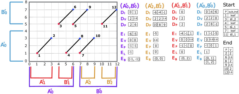
Fig 4. Visualization of subproblems divisions.

The data structures needed for each subproblem: D_I, D_V, D_P, E_I, E_V, E_P, E_L and E_B after the processing of all the 12 points. Points are numbered in the order of processing (Cartesian sorted order). 12 points are assigned into three column subproblems $(A_0^c,B_0^c)$, $(A_1^c,B_1^c)$, $(A_2^c,B_2^c)$ and one row subproblem $(A_0^r,B_0^r)$, where starting points are assigned to A-part and endpoints are assigned to B-part. Leaf subproblems are not shown for simplicity. Start and End are used for the traceback of the optimal chain. Start stores sub—the index of the subproblem which yields the optimal chaining score up to a starting point and ind—φ(E_I, f_i), where f_i is the diagonal of the starting point. End stores the optimal value for each endpoint. For this toy example, the match bonus of every fragment is 2 and the gap cost function of appending fragment α_j to fragment α_i is $gap({\alpha }_i,{\alpha }_j)=0.25*log\left(\right|(y_i^e-x_i^e)-(y_j^s-x_j^s)+1\left|\right)+1$, where $(x_i^e,y_i^e)$ is the endpoint of α_i and $(x_j^s,y_j^s)$ is the starting point of α_j. End indicates that there are three optimal chains achieving the optimal value: 2.8. By tracing back, chain-1: point-1, point-2, point-3, point-6, chain-2: point-1, point-2, point-5, point-9 and chain-3: point-7, point-10, point-11, point-12.