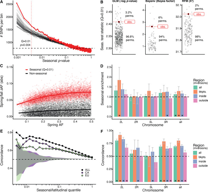
Figure 2. Signals of seasonal adaptation.

(A) p-value distribution of GLM seasonal regression (red line), permutations (solid black lines, 50/500 plotted), and expected values (dashed black line). (B) Comparison of seasonal test statistics (quantile = 0.01) for observed (red) and permuted (black) datasets, for the three analyses: i: GLM (−log p-value), ii: Bayenv (Bayes factor; outlier of a Bayes factor of 10 excluded from plotting), iii: RFM (X²). (C) Average spring/fall allele frequency change for each of the top 1% of seasonally varying SNPs (red) and non-seasonal, matched control SNPs (black), as a function of the folded spring allele frequency. Lines represent a moving average across SNPs with a given spring allele frequency. (D) Enrichment of seasonal SNPs (median of 500 permutations). Enrichment is calculated as the observed number of seasonal SNPs over the number of seasonal SNPs in each permutation at p<0.004. The genome is subset by chromosome and location relative to major cosmopolitan inversions (bkpts.: inversion breakpoints ± 1 Mb, inside: interior to the breakpoints excluding 1 Mb buffer, outside: exterior to the breakpoints excluding the 1 Mb buffers). Error bars are 95% confidence intervals and asterisks denote greater seasonal enrichment than more than 95% of permutations. (E, F) Concordance rates of seasonal and clinal polymorphisms by (E) geographic region and (F) genomic region. The y-axis represents the concordance rate of allele frequency change across time and space, assuming that the winter favored allele is the same as the allele favored in high latitudes. Clinal polymorphisms were identified along the East Coast of North America. Seasonal sites were identified using all populations not used in the clinal analysis (n = 18). (E) Seasonal sites were also identified using exclusively the California populations (purple: n = 3) or the Europe populations (green: n = 3). Shaded areas are the 95% confidence intervals of 100 matched control datasets for the Californian (purple) and European (green) analyses. (F) Concordance by genomic region. Error bars are 95% confidence intervals (binomial error) and asterisks denote concordance significantly greater than 0.5 (binomial test p<0.05).

Figure 2—figure supplement 1. Enrichment of seasonal SNPs by chromosome and significance threshold.

Enrichment is calculated as the observed number of seasonal SNPs over the number of seasonal SNPs in each permutation (median of 500 permutations). Error bars are 95% confidence intervals, and asterisks denote greater seasonal enrichment than more than 95% of permutations.

Figure 2—figure supplement 2. Comparison of bayenv and GLM seasonal analyses.

(A) Proportion of SNPs found highly seasonal in both the GLM and the bayenv seasonal analyses. (B) Seasonal and latitudinal concordance for both the GLM and the bayenv analyses.

Figure 2—figure supplement 3. Artificial sample size increases for GLM and RFM methods.

The effect of artificial increases of sample size on the Core20 seasonal analysis using (A, C) the RFM and (B, D) the GLM analyses. Top row: sample size inflated by a fixed amount. Bottom row: sample size inflated by a Poisson sampled amount. Shown is the proportion of SNPs in each bin (solid lines) compared with the null expectation (dashed line). Black: original dataset. Dark gray: 10 reads added to each sample (same allele frequencies). Light gray: 100 reads added to each sample (same allele frequencies).

Figure 2—figure supplement 4. Comparison of the GLM and the Bayenv model for assessing clinal and seasonal concordance.

(A) The ‘joint quantile threshold’ is the quantile threshold for both the seasonal and the clinal analysis, and includes all SNPs at that quantile or less. (B) The ‘joint quantile bin’ includes only those SNPs at that specific quantile.