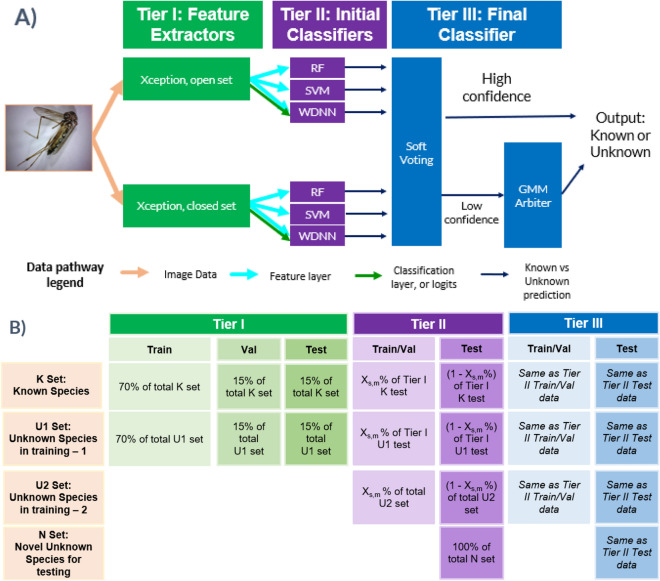
Figure 2.

The novelty detection architecture was designed with three tiers to assess whether the CNNs were familiar with the species shown in each image. (A) Tier I consisted of two CNNs used as feature extractors. Tier II consisted of initial classifiers making an initial determination about whether the specimen is known or unknown by analyzing the features of one of the Tier I CNNs, and the logits in the case of the wide and deep neural network (WDNN). In this figure, SVM refers to a support vector machine, and RF refers to a random forest. Tier III makes the final classification, first with soft voting of the Tier II outputs, then sending high confidence predictions as the final output and low confidence predictions to a Gaussian Mixture Model (GMM) to serve as the arbiter for low confidence predictions. (B) Data partitioning for training each component of the architecture is summarized: Tier I is trained on the K set of species, known to the algorithm; Tier I open-set CNN is also trained on the U1 set of species, the first set of unknown species used in training; Tier II is trained on K set, U1 set, and the U2 set of species, the second set of unknown species used in training; Tier III is trained on the same species and data-split as Tier II. Data-split ratios were variable for each species over each iteration (X_s,m where s represents a species, m represents a fold, and X is a percentage of the data devoted to training) for Tiers II and III; X_s,m was adjusted to manage class imbalance within genus across known and unknown classes. Testing was performed on each of the K, U1, and U2 sets, as well as the N set, the final set of unknown species reserved for testing the algorithm, such that it is tested on previously unseen taxa, replicating the plausible scenario to be encountered in deployment of CNNs for species classification. Over the twenty-five folds, each known species was considered unknown for at least five folds and included as novel for at least one-fold.