Figure - PMC

Skip to main content

An official website of the United States government

Here's how you know

Here's how you know

Official websites use .gov
A .gov website belongs to an official government organization in the United States.

Secure .gov websites use HTTPS
A lock ( ) or https:// means you've safely connected to the .gov website. Share sensitive information only on official, secure websites.

View full-text article in PMC

. 2021 Jun 21;15:691821. doi: 10.3389/fnhum.2021.691821

Search in PMC
Search in PubMed
View in NLM Catalog
Add to search

Copyright © 2021 Gordon, Dörre, Belardinelli, Stenroos, Zrenner, Ziemann and Zrenner.

This is an open-access article distributed under the terms of the Creative Commons Attribution License (CC BY). The use, distribution or reproduction in other forums is permitted, provided the original author(s) and the copyright owner(s) are credited and that the original publication in this journal is cited, in accordance with accepted academic practice. No use, distribution or reproduction is permitted which does not comply with these terms.

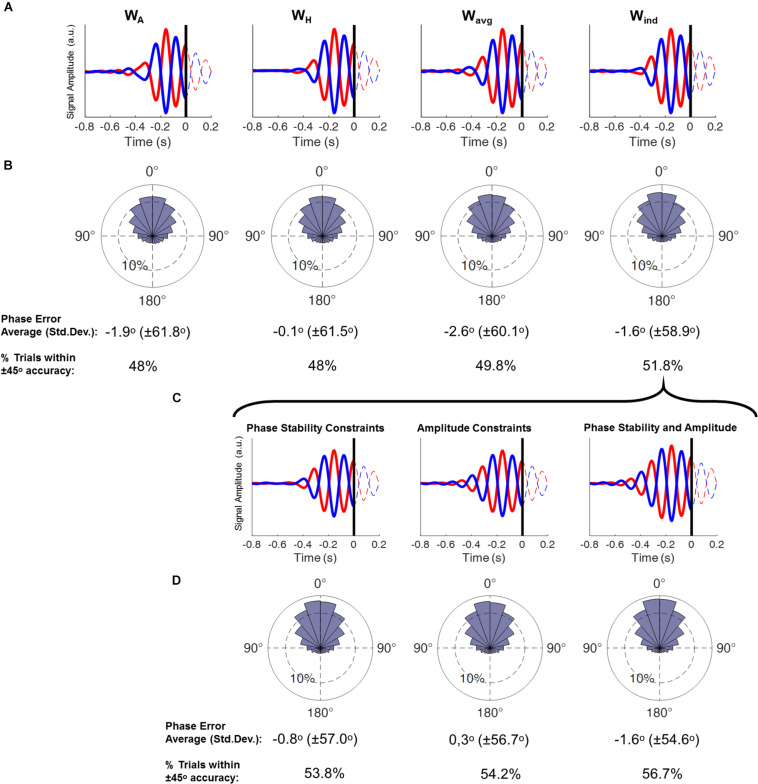
PMC Copyright notice

(A) Time course plots display the averaged epochs obtained by running the real-time phase detection algorithm with resting-state EEG, with data obtained by using each spatial filter. Here only trials that were classified as positive peak (red) and negative peak (blue) were included. Time = 0 refers to the time point the theta phase was being estimated. Columns display the results from each spatial filter. (B) Phase histograms show the accuracy of the phase estimation from each spatial filter, obtained by subtracting the estimated phase of all epochs by their corresponding “gold-standard” phase (phase-bin width 20°, inner ring corresponds to 10% of the total trials). Below are the circular averages and standard deviations of the results, and the proportion of epochs within ± 45° accuracy (ANOVA, p = 0.0025; post-hoc W_A = W_H < W_avg < W_ind). (C) Time course plots display the averaged epochs obtained by running the real-time phase detection algorithm with resting-state EEG (as in A), with data obtained by using the W_ind filter and followed by different signal constraints: Phase stability, signal amplitude and both phase stability and amplitude constraints. (D) Phase histograms show the accuracy of the phase estimation (as in B) from the signal after application of each constraint (ANOVA, p = 0.0002; post-hoc [NO constraints] < [phase stability] = [amplitude] < [phase stability AND amplitude]).