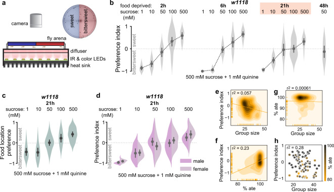
Fig. 1. Hungry flies make trade-offs between the appetitive and aversive value of food.

a Schematic of the two-choice decision making assay. Sweet and bittersweet foods are prepared in dissolved agarose, mixed with food dyes, and gelled in a circular arena. Flies are introduced into the dark food arena to walk and consume freely for 5 min. Flies are then anaesthetized and abdomen color is recorded, indicating ingested food choice. Preference index is calculated as (no. of sweet color flies + 0.5 purple flies) − (no. of bittersweet color flies + 0.5 purple flies)/total no. of flies that ate, where positive index means flies preferred sweet and negative index means flies preferred bittersweet. b Preference index of wild-type (w1118) flies deprived of food for increasing durations indicate the tradeoff between the sweet and bittersweet food and reveal equal preference when the choice is between 50 mM sucrose-only and 500 mM sucrose + 1 mM quinine. c Position preference index (i.e., sweet or bittersweet sector preference as defined by the location of the flies at the end of the assay) matches ingested food preference. d Preferences of male and female flies within each group were indistinguishable for all conditions tested. There was no significant correlation between preference index and group size per trial (e), preference index and % of flies that ate per trial (f) or % of flies that ate per trial and group size (g). h Neither group size nor % flies that ate significantly predicted preference index in a multiple regression model, indicating no interaction between these measures. b–d Plots show mean ± 95% CI, violins depict kernel density estimation of the underlying data distribution with the width of each violin scaled by the number of observations at that y-value. Each violin summarizes 10 ≤ trials ≤ 30 with mode = 10. e–h Heatmaps depict bivariate distribution visualized using a kernel density estimation procedure; darker regions indicate higher data density. r² is the square of Pearson’s coefficient. See Supplementary Table 1 for sample size and statistics. Nonsignificant differences are not depicted in figures.