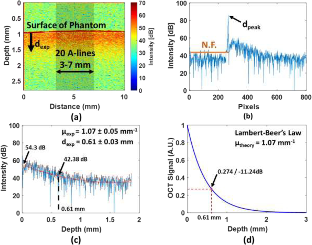
Fig. 4.

A homogeneous phantom testing and a numerical simulation with finite depth. (a) shows the OCT image of a homogeneous phantom. (b) represents an example of averaged 20 A-scan signals (the waveform in blue) and the N.F. (the solid line in orange). (c) The quadratic polynomial curve fitting (red line) was used to fit 20 individual A-scan signals. (d) A result from the numerical simulation based on Lambert-Beer’s Law.
