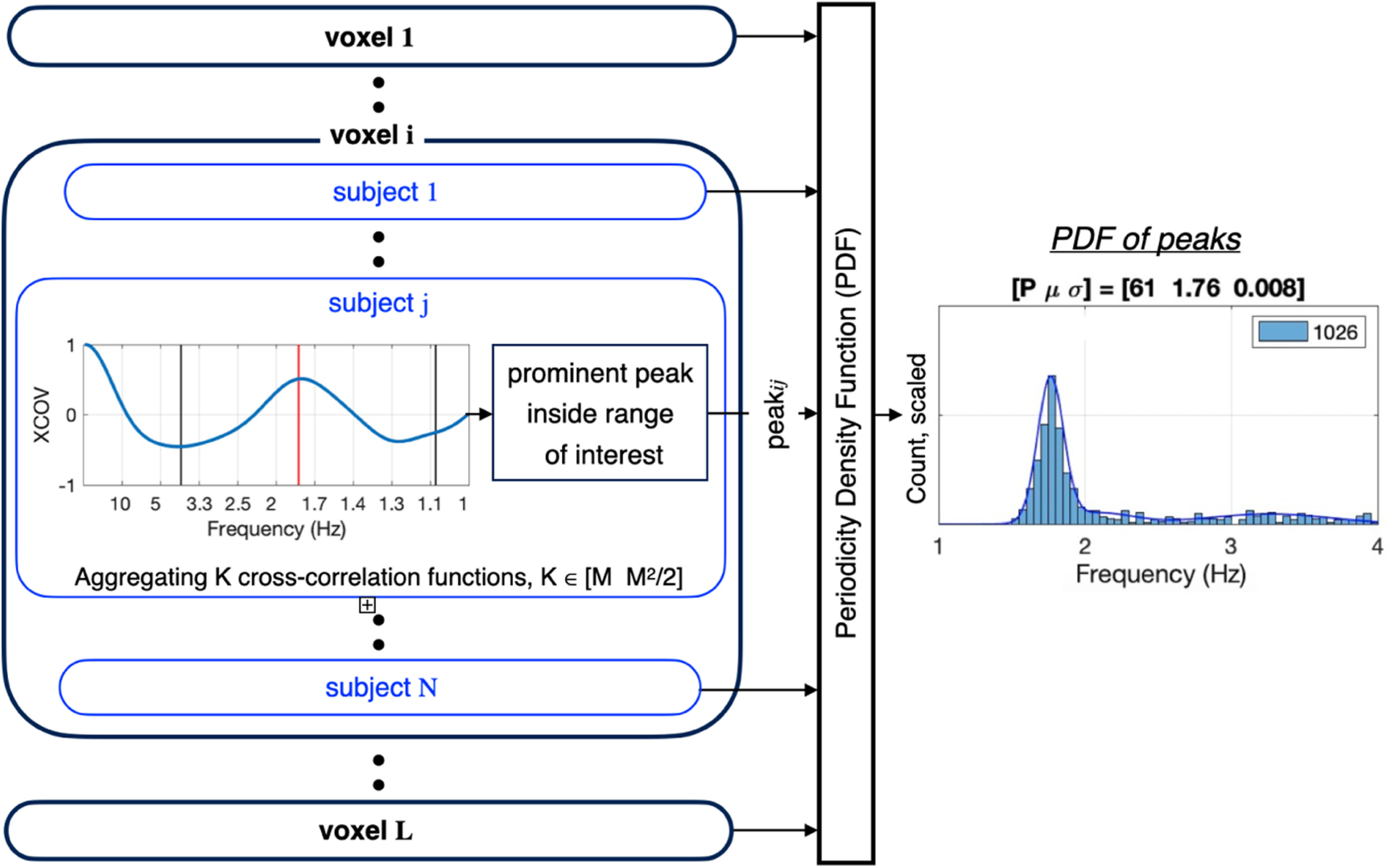
Figure 3.

Analysis pipeline for deriving the PDF within a particular ROI. Shown is the resulting periodicity density function (PDF) for a given condition (say, the 1.8-Hz condition), a given response class (say, hit), and a given region of interest (ROI; say, STG). L voxels, N subjects, and M trials per subject are considered. For the i-th voxel and the j-th subject, periodicity is computed using a newly proposed measure method termed XCOV. First (data not shown), each brain signal is filtered to the frequency range of interest. Cross-correlations were computed using the filtered signals. Note that as a cross-correlation function, XCOV is computed against time-lags; the abscissa here shows the time-lag inverse, in frequency, hence going from right to left. The PDF is derived by (1) forming a histogram of the XCOV peak locations inside the frequency range of interest; (2) normalizing the histogram to L × N, the total number of data points; and (3) building a third order Gaussian Mixture Model (GMM) that fits the histogram. The GMM model is the desired PDF. The goodness of the PDF is quantified by in terms of p value, the percentage of datapoints inside the frequency range of interest with respect to the total number of datapoints (L × N); and the mean μ and variance σ of the prominent Gaussian component of a third order GMM. (The total number of data points is shown in the inset of each entry.)