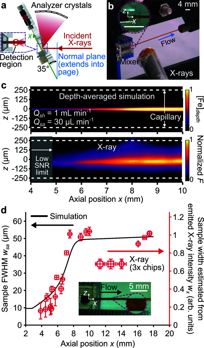
Figure 4.

Experimental setup at the X-ray beamline and comparison with simulations. (a) Schematic of mixer placed at a 35° angle to the incident X-rays. (b) Mixer mounted on the beamline plate during X-ray operation. (c) Line-of-sight integrated profile of predicted axisymmetric concentration fields for all Fe species (top row) and measured Fe X-ray fluorescence (bottom row). The gray area in the X-ray image depicts the region where the sample stream cross-sectional area is too small for X-ray detection. Note that the convolutive effect of the X-ray beam significantly widens the apparent sample. (d) The left ordinate (corresponding to the line) is the predicted sample FWHM w _sa and the right ordinate (corresponding to the symbols) is the sample width associated with the emitted X-ray intensities w _x . Both quantities are plotted versus the axial position x and data are for the same flow conditions as (c). The vertical and horizontal uncertainty bars, respectively, correspond to the standard deviation of w _x among four different methods of measuring the emitted X-ray intensity and the X-ray beam FWHM along x. The inset shows the experimental device and a zoomed-in view of an example X-ray mark on the polyimide capillary.