
Figure 3.
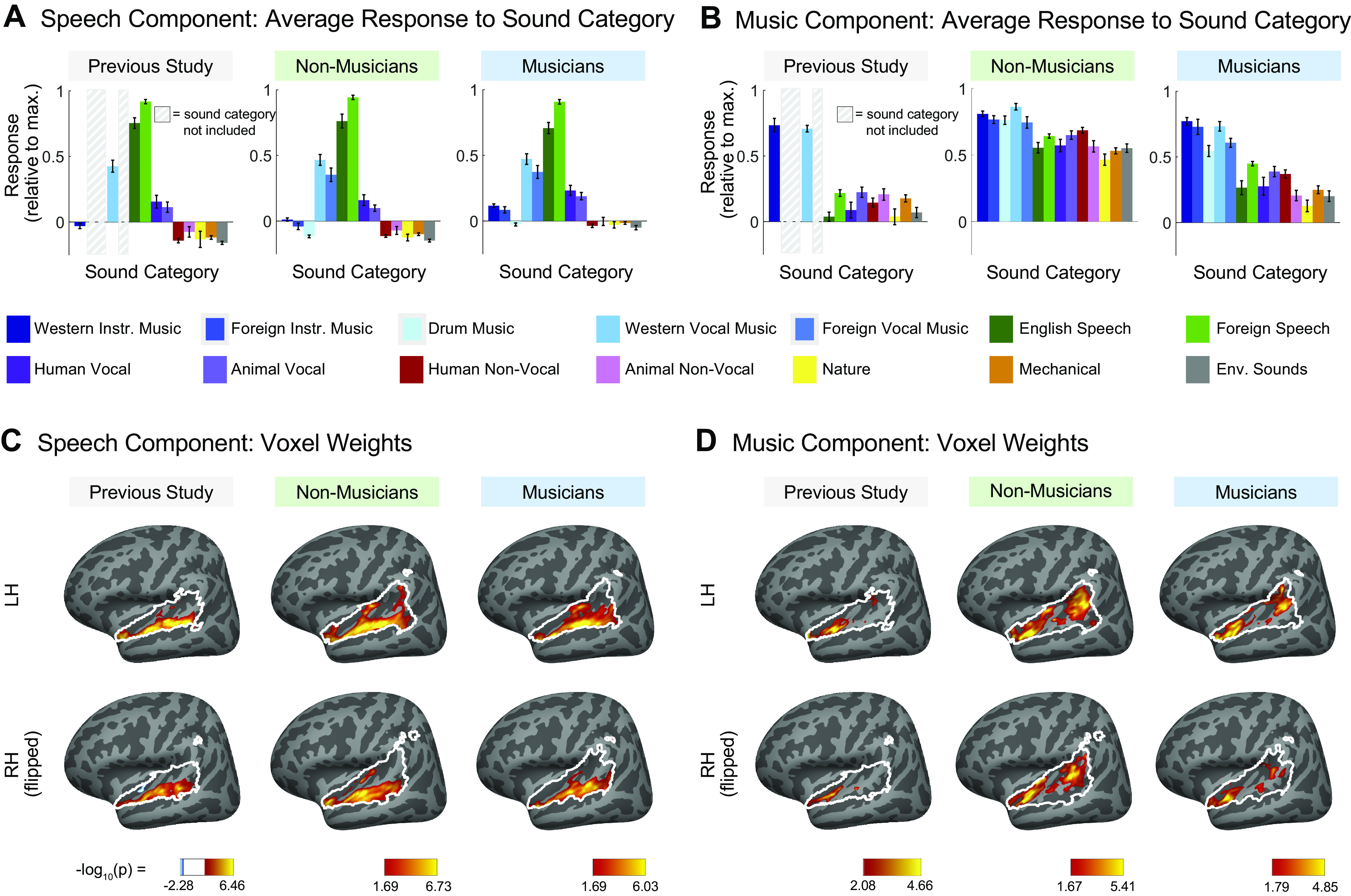
Comparison of speech-selective and music-selective components for participants from previous study (n = 10), nonmusicians (n = 10), and musicians (n = 10). A and B: component response profiles averaged by sound category (as determined by raters on Amazon Mechanical Turk). A: the speech-selective component responds highly to speech and music with vocals, and minimally to all other sound categories. Shown separately for the previous study (left), nonmusicians (middle), and musicians (right). Note that the previous study contained only a subset of the stimuli (165 sounds) used in the current study (192 sounds) so some conditions were not included and are thus replaced by a gray rectangle in the plots and surrounded by a gray rectangle in the legend. B: the music-selective component (right) responds highly to both instrumental and vocal music, and less strongly to other sound categories. Note that “Western Vocal Music” stimuli were sung in English. We note that the mean response profile magnitude differs between groups, but that selectivity as measured by separability of music and nonmusic is not affected by this difference (see text for explanation). For both A and B, error bars plot one standard error of the mean across sounds from a category, computed using bootstrapping (10,000 samples). C: spatial distribution of speech-selective component voxel weights in both hemispheres. D: spatial distribution of music-selective component voxel weights. Color denotes the statistical significance of the weights, computed using a random effects analysis across subjects comparing weights against 0; P values are logarithmically transformed (−log10[P]). The white outline indicates the voxels that were both sound-responsive (sound vs. silence, P < 0.001 uncorrected) and split-half reliable (r > 0.3) at the group level (see materials and methods for details). The color scale represents voxels that are significant at FDR q = 0.05, with this threshold computed for each component separately. Voxels that do not survive FDR correction are not colored, and these values appear as white on the color bar. The right hemisphere (bottom rows) is flipped to make it easier to visually compare weight distributions across hemispheres. Note that the secondary posterior cluster of music component weights is not as prominent in this visualization of the data from Ref. 7 due to the thresholding procedure used here; we found in additional analyses that a posterior cluster emerged if a more lenient threshold is used. FDR, false discovery rate; LH, left hemisphere; RH, right hemisphere.